Introduction to Self-Organizing Maps in Multi-Attribute Seismic Data

Abstract

Unsupervised neural network searches multi-dimensional data for natural clusters. Neurons are attracted to areas of higher information density. The SOM analysis relates to subsurface geometry and rock properties while noting multi-attribute seismic properties at the wells, correlating to rock lithologies, with those away from the wells.

Computers that think like a human are well beyond our current capabilities but computers that learn are not. They are around us every day. Pocket cameras identify faces in a live digital image and automatically adjust the focus when the shutter is pressed. Post offices scan the mail and route the documents appropriately. Offices scan documents as bitmaps and convert them to text documents for editing. Web documents are indexed for content, while search engines deliver these documents through key word searches in unprecedented detail and with extraordinary speed.

We have seen a tremendous growth in the size of 3D survey seismic data volumes, and it is common today for both 2D and 3D seismic surveys to be integrated into the interpretation. Moreover, the primary survey of reflection amplitude is interpreted along with derived surveys of perhaps 5 to 25 attributes. The attributes of both 2D and 3D surveys represent multidimensional data. The problem is to keep all this data in one’s head while trying to find oil and gas. Much interpretation effort is devoted to building a geologic framework from the seismic data, identifying key reflecting intervals where oil and gas might be found and finding an interesting anomaly. At this point attributes are the framework in which we evaluate the anomaly. But this is the point where we can easily mislead ourselves. It is quite easy to build a plausible model for a prospect using only those attributes which fit our model and ignore the rest. This is bad enough, but there is even a greater crime. Lurking in the data may be combinations of attributes which are legitimate anomalies but which are never found at all.

Learning machines are artificial neural networks which can construct an experience data base from multidimensional data such as multi-attribute seismic surveys. There are two main classes of neural networks – supervised and unsupervised. With supervised neural networks, a network classifies data into groups sharing given characteristics that have already been classified by an expert. After careful processing, synthetic seismograms that are prepared at well sites serve as the expert’s data. Then the neural network is trained to classify these data at the wells. After training, the neural network literally roams the seismic data to classify areas which might be similar in some given sense to models developed at the well locations.

Alternatively, an unsupervised neural network searches multidimensional data for natural clusters. Neurons are attracted to areas of higher information density. The most popular unsupervised neural network, self-organizing maps (SOM), were introduced by Teuvo Kohonen in 1981 [1]. SOM was successfully applied to seismic facies analysis by Poupon, Azbel and Ingram in 1999 (Stratimagic) [2]. We preface recent efforts to bring SOM to bear on multiattribute seismic interpretation with a simple SOM example used by Kohonen to illustrate some of its basic features.

Quality of Life

An early problem considered by Kohonen and his research team was to identify natural clusters as they relate to quality of life factors based on World Bank data. A study that included 126 countries, considered a total of 39 measurements describing the level of poverty found in each country. While the data matrix was somewhat limited by incomplete reporting, the SOM results are still quite interesting. Shown in Figure 1 is the SOM which resulted from the learning process. Canada (CAN) and the United States of America (USA) clustered at the same neuron location shown at the 6th row of the 1st column in the figure. Ethiopia (ETH) is found on the right edge at column 13, row 5. Other country abbreviations and further details are in [3].

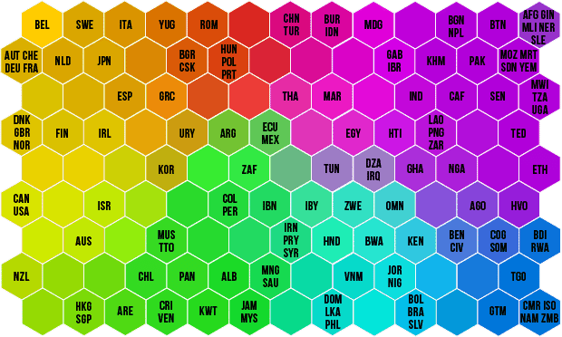
The reason that countries of similar quality of life cluster in similar neuron areas has to do with learning principles that are built into SOM. In this study, every country is a sample and that sample is a column vector of 39 elements. In other words, there are 39 attributes in this problem. Countries of similar characteristics (a natural cluster) plot in about the same place in attribute space. At the beginning of the learning process, neurons of 39 dimensions are assigned random numbers. During the learning process, the neurons move toward natural clusters. The data points never move. The mathematics of SOM learning define both competitive and cooperative learning. For a given data sample, the Euclidean distance is computed between the sample and each neuron. The neuron which is “nearest” to the data sample is declared the “winning” neuron and allowed to advance a fraction of the distance toward the data sample. The neuron movement is the essence of machine learning. Competitive learning is embodied in the strategy that the winning neuron moves toward the data sample.

This aspect of cooperative learning is related to the layout of the neural network. In SOM learning, the neural network is commonly a 2D hexagonal grid. This constitutes the neuron topology; the choice of a hexagonal grid rather than a rectangular grid will be apparent shortly. When a winning neuron has been found, cooperative learning takes place because the neurons in the vicinity of the winning neuron (the neighborhood) are also allowed to move toward the data sample, but by an amount less than the winning neuron. In fact, the further a neighborhood is away from the winning neuron, the less it is allowed to move. Hexagonal grids move more neurons than rectangular grids because they have 6 points of contact with their immediate neighbors instead of 4. Learning continues as winning and neighborhood neurons move toward each sample in turn until the entire set of samples has been processed. At this point, one epoch of learning has been completed. The event is marked as one time step in the learning process. For each subsequent epoch the distance a winning neuron may move toward a data sample is reduced slightly and the size of the neighborhood is also reduced. The learning process terminates when there is no further appreciable movement of the neurons. Often the number of such epochs can be in the hundreds or thousands.

As demonstrated in Figure 1, natural clustering of like-quality of life countries arises from both competitive and cooperative learning. But one may ask how is SOM learning unsupervised when the SOM map displays country labels? The answer is that in the steps just described, there is no need to order the sequence of samples in the SOM learning process. The Ethiopia sample may be processed between samples for Canada and USA with no effect on the outcome. The sample order of countries may be scrambled randomly.

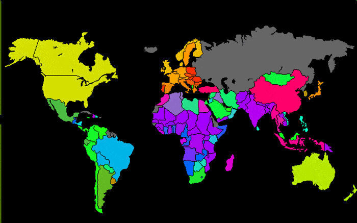
In Kohonen’s analysis of the World Bank data, the names of countries are known, however. When the SOM learning process is completed, the neuron which is closest to each country sample is labeled by the country label as shown in Figure 1. The neuron colors are arbitrary. Figure 2 is a world map in which each country is colored with the color scale used in Figure 1. Countries with similar quality of life are therefore colored similarly. Several countries which did not contribute data for the report are colored gray (Russia, Iceland, Cuba and several others). Figure 2 illustrates how the results of neural network analysis are used to classify the data. We shall see in the next section how SOM analysis and classification is an important addition to seismic interpretation.

Gulf of Mexico Salt Dome Survey

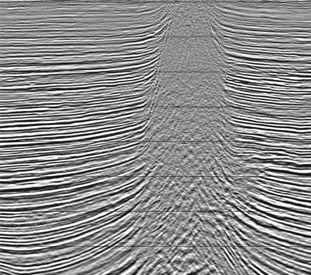
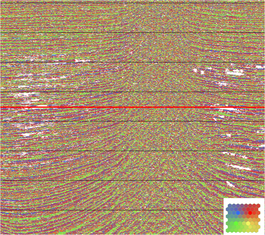
A SOM analysis was conducted on a 3D survey in the Gulf of Mexico provided by FairfieldNodal. See [4] for a description of SOM theory and a discussion of the processing steps. In particular, the introduction of a so-called curvature measure and the harvesting process are particularly relevant. Figure 3 is a vertical amplitude section across the center of the salt. Figure 4 shows the SOM analysis of 13 attributes across the same location. The SOM map is a 2D colorbar based on an 8 x 8 hexagonal grid. There are 100 epochs in the present analysis. It is readily apparent that the SOM classification is tracking seismic reflections.

Shown in Figure 4 are white portions in which data have been “declassified”, a concept which we now explain. After the SOM analysis is completed, every sample in the survey is associated with a winning neuron. This implies that every neuron is associated with a given set of samples.

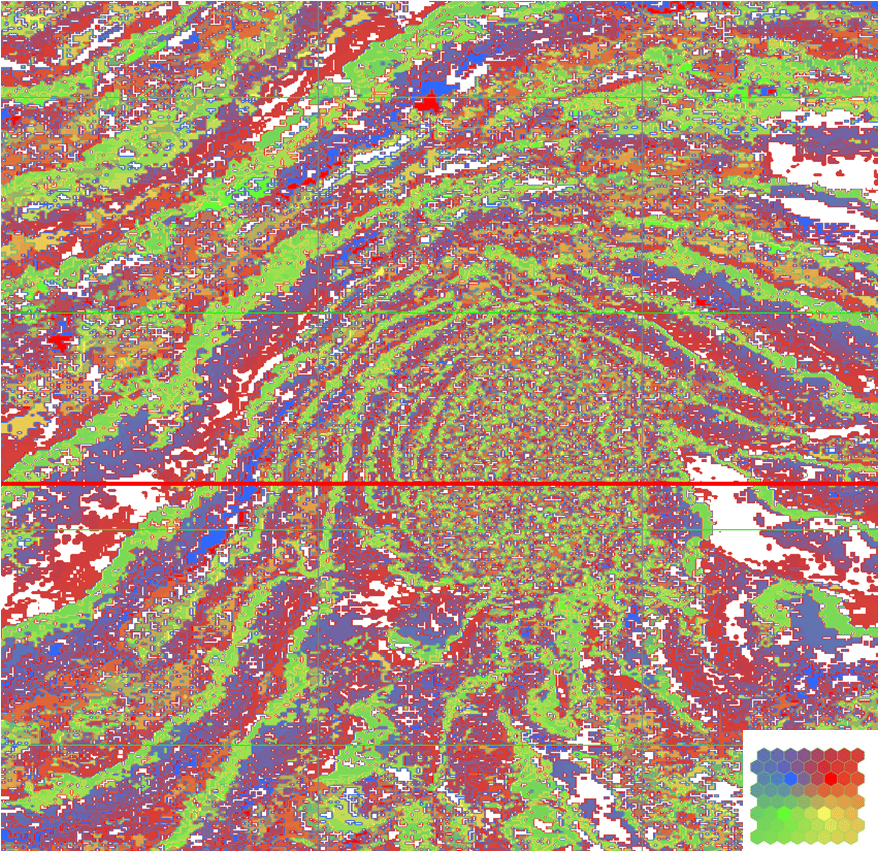
For any particular neuron, some samples are nearby in attribute space and others are far away. This means that there is a statistical population of distances on which to declassify what we shall call “outliers”. When a neuron is near a data sample, the probability that the sample is correctly classified is high. If a neuron and sample coincide, the probability is 100%. In Figure 4, those samples for which the probability is less than 10% are not assigned any classification. We identify such outliers as SOM anomalies. SOM anomalies are scattered about the section, with several which are larger and more compact. The horizontal red line marks the time of the time slice shown in Figure 5.

The horizontal line in Figure 5 marks the location of the section in Figure 4. Notice the white area to the right of the salt dome crossed by the red line in Figure 4 is identified as the same white area right of the salt dome and crossed by the red line in Figure 5. We note that the SOM anomaly is a discrete geobody which appears to be related to the upturned beds flanking the salt. By geobody, we mean a contiguous region of samples in the survey which share some characteristic.

Wharton County Survey

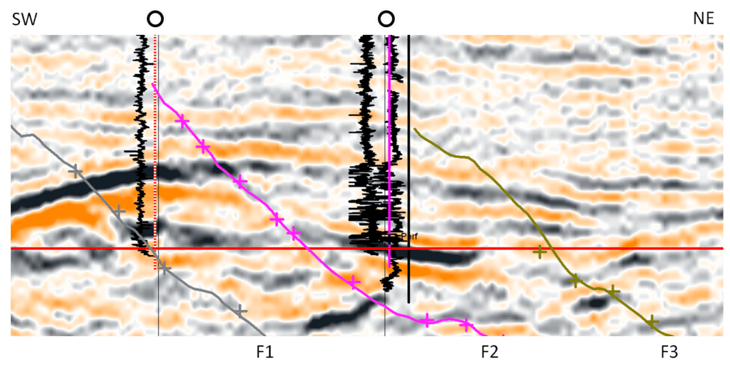
A SOM analysis was also conducted on a 3D survey in Wharton County, Texas provided by Auburn Energy. Details of this study are found in [5]. An arbitrary line through the survey between two wells is shown in Figure 6.
The well at the left presented a gas show while the well at the right developed a single-well gas field. Note the association of gas with faults F1, F2 and F3.

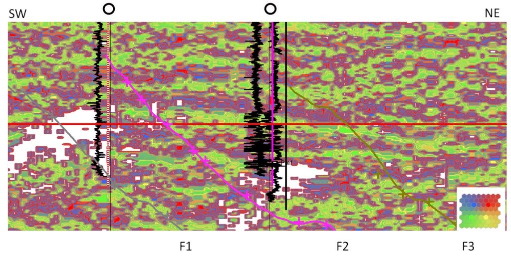
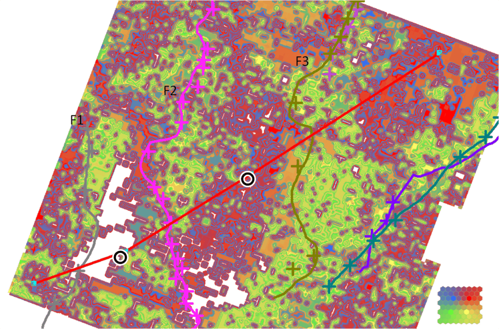
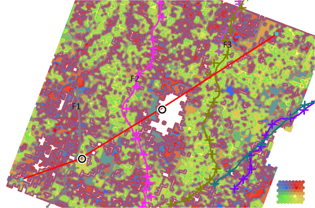
Figure 7 shows a portion of the results of a SOM classification run designed in the same way as in the previous example, namely by use of the same 13 attributes, an 8 x 8 hexagonal topology of neurons and a probability cut-off of 10%. Notice that this selection of attributes did not delineate the faults very well, yet SOM anomalies are found near both wells. The time slice of Figure 8 confirms that the SOM anomaly to the left of the gas-show well (left) is a geobody. A smaller second SOM anomaly is shown right of the F2 fault. Figure 9 is a time slice through the lower SOM anomaly near the gas well (right) of Figure 7. Notice that it too is a geobody. Prior to the present SOM analysis, an earlier thorough interpretation had been conducted with all available geophysical and geological data. A large set of attributes was used, including AVO gathers, offset stacks, advanced processing as well as some proprietary attributes. As a result, four wells were drilled. Two wells had no gas shows and are not marked here. No SOM anomaly was found at or near either of the two dry wells.

Further Work

The next step in this work is to gain a better understanding how the patterns obtained with SOM analysis relate to subsurface geometry and its rock properties. Research is currently underway in an attempt to answer questions of this kind. It is also important to further address the relationship between multi-attribute seismic properties at the wells, which correlate to rock lithologies, with those away from the wells.

Conclusion

Computerized information management has become an indispensable tool for organizing and presenting geophysical and geological data for seismic interpretation. Databases provide the underlying environment to achieve this goal. Machine learning is another area in which computers may one day offer an indispensable tool as well. The point is particularly germane in light of successes achieved by machine learning in other fields. The engines to help us reach this objective could well be neural networks that adapt to the data and present its various structures in a way that is meaningful to the interpreter. We believe that neural networks offer many advantages which our industry is just now recognizing.

References

Kohonen, T., 2001, Self-Organizing Maps, 3rd edition: Springer
Poupon, M., Azbel K. and Ingram, J., 1999, Integrating seismic facies and petro-acoustic modeling:
World Oil Magazine, June, 1999, http://www.cis.hut.fi/research/som-research/worldmap.html accessed 10 November, 2010
Smith, T. and Treitel, S., 2010, Self-organizing artificial neural nets for automatic anomaly identification: SEG International Convention (Denver) Extended Abstracts
Smith, T., 2010, Unsupervised neural networks – disruptive technology for seismic interpretation: Oil & Gas Journal, Oct. 4, 2010