Geologic Pattern Recognition from Seismic Attributes: Principal Component Analysis and Self-Organizing Maps

Abstract

Interpretation of seismic reflection data routinely involves powerful multiple-central-processing-unit computers, advanced visualization techniques, and generation of numerous seismic data types and attributes. Even with these technologies at the disposal of interpreters, there are additional techniques to derive even more useful information from our data. Over the last few years, there have been efforts to distill numerous seismic attributes into volumes that are easily evaluated for their geologic significance and improved seismic interpretation. Seismic attributes are any measurable property of seismic data. Commonly used categories of seismic attributes include instantaneous, geometric, amplitude accentuating, amplitude-variation with offset, spectral decomposition, and inversion. Principal Component Analysis (PCA), a linear quantitative technique, has proven to be an excellent approach for use in understanding which seismic attributes or combination of seismic attributes has interpretive significance. The PCA reduces a large set of seismic attributes to indicate variations in the data, which often relate to geologic features of interest. PCA, as a tool used in an interpretation workflow, can help to determine meaningful seismic attributes. In turn, these attributes are input to self-organizing-map (SOM) training. The SOM, a form of unsupervised neural networks, has proven to take many of these seismic attributes and produce meaningful and easily interpretable results. SOM analysis reveals the natural clustering and patterns in data and has been beneficial in defining stratigraphy, seismic facies, direct hydrocarbon indicator features, and aspects of shale plays, such as fault/fracture trends and sweet spots. With modern visualization capabilities and the application of 2D color maps, SOM routinely identifies meaningful geologic patterns. Recent work using SOM and PCA has revealed geologic features that were not previously identified or easily interpreted from the seismic data. The ultimate goal in this multiattribute analysis is to enable the geoscientist to produce a more accurate interpretation and reduce exploration and development risk.

Introduction

The object of seismic interpretation is to extract all the geologic information possible from the data as it relates to structure, stratigraphy, rock properties, and perhaps reservoir fluid changes in space and time (Liner, 1999). Over the past two decades, the industry has seen significant advancements in interpretation capabilities, strongly driven by increased computer power and associated visualization technology. Advanced picking and tracking algorithms for horizons and faults, integration of prestack and poststack seismic data, detailed mapping capabilities, integration of well data, development of geologic models, seismic analysis and fluid modeling, and generation of seismic attributes are all part of the seismic interpreter’s toolkit. What is the next advancement in seismic interpretation? A significant issue in today’s interpretation environment is the enormous amount of data that is used and generated in and for our workstations. Seismic gathers, regional 3D surveys with numerous processing versions, large populations of wells and associated data, and dozens if not hundreds of seismic attributes, routinely produce quantities of data in terms of terabytes. The ability for the interpreter to make meaningful interpretations from these huge projects can be difficult and at times quite inefficient. Is the next step in the advancement of interpretation the ability to interpret large quantities of seismic data more effectively and potentially derive more meaningful information from the data?

For example, is there a more efficient methodology to analyze prestack data whether interpreting gathers, offset/angle stacks, or amplitude-variation with offset (AVO) attributes? Can the numerous volumes of data produced by spectral decomposition be efficiently analyzed to determine which frequencies contain the most meaningful information? Is it possible to derive more geologic information from the numerous seismic attributes generated by interpreters by evaluating numerous attributes all at once and not each one individually? This paper describes the methodologies to analyze combinations of seismic attributes of any kind for meaningful patterns that correspond to geologic features. Principal component analysis (PCA) and self organizing maps (SOMs) provide multiattribute analyses that have proven to be an excellent pattern recognition approach in the seismic interpretation workflow. A seismic attribute is any measurable property of seismic data, such as amplitude, dip, phase, frequency, and polarity that can be measured at one instant in time/depth over a time/depth window, on a single trace, on a set of traces, or on a surface interpreted from the seismic data (Schlumberger Oilfield Glossary, 2015). Seismic attributes reveal features, relationships, and patterns in the seismic data that otherwise might not be noticed (Chopra and Marfurt, 2007). Therefore, it is only logical to deduce that a multiattribute approach with the proper input parameters can produce even more meaningful results and help to reduce risk in prospects and projects.

Evolution of seismic attributes

Balch (1971) and Anstey at Seiscom-Delta in the early 1970s are credited with producing some of the first generation of seismic attributes and stimulated the industry to rethink standard methodology when these results were presented in color. Further development was advanced with the publications by Taner and Sheriff (1977) and Taner et al. (1979) who present complex trace attributes to display aspects of seismic data in color not seen before, at least in the interpretation community. The primary complex trace attributes including reflection strength/envelope, instantaneous phase, and instantaneous frequency inspired several generations of new seismic attributes that evolved as our visualization and computer power improved. Since the 1970s, there has been an explosion of seismic attributes to such an extent that there is not a standard approach to categorize these attributes. Brown (1996) categorizes seismic attributes by time, amplitude, frequency, and attenuation in prestack and poststack modes. Chen and Sidney (1997) categorize seismic attributes by wave kinematics/dynamics and by reservoir features. Taner (2003) further categorizes seismic attributes by prestack and by poststack, which is further divided into instantaneous, physical, geometric, wavelet, reflective, and transmissive. Table 1 is a composite list of seismic attributes and associated categories routinely used in seismic interpretation today. There are of course many more seismic attributes and combinations of seismic attributes than listed in Table 1, but as Barnes (2006) suggests, if you do not know what an attribute means or is used for, discard it. Barnes (2006) prefers attributes with geologic or geophysical significance and avoids attributes with purely mathematical meaning. In a similar vein, Kalkomey (1997) indicates that when correlating well control with seismic attributes, there is a high probability of spurious correlations if the well measurements are small or the number of independent seismic attributes is considered large. Therefore, the recommendation when the well correlation is small is that only those seismic attributes that have a physically justifiable relationship with the reservoir property be considered as candidates for predictors.

In an effort to improve the interpretation of seismic attributes, interpreters began to coblend two and three attributes together to better visualize features of interest. Even the generation of attributes on attributes has been used. Abele and Roden (2012) describe an example of this where dip of maximum similarity, a type of coherency, was generated for two spectral decomposition volumes high and low bands, which displayed high energy at certain frequencies in the Eagle Ford Shale interval of South Texas. The similarity results at the Eagle Ford from the high-frequency data showed more detail of fault and fracture trends than the similarity volume of the full-frequency data. Even the low-frequency similarity results displayed better regional trends than the original full-frequency data. From the evolution of ever more seismic attributes that multiply the information to interpret, we investigate PCA and self organizing maps to derive more useful information from multiattribute data in the search for oil and gas.

Principal component analysis

PCA is a linear mathematical technique used to reduce a large set of seismic attributes to a small set that still contains most of the variation in the large set. In other words, PCA is a good approach to identify the combination of most meaningful seismic attributes generated from an original volume. The first principal component accounts for as much of the variability in the data as possible, and each succeeding component (orthogonal to each preceding) accounts for as much of the remaining variability (Guo et al., 2009; Haykin, 2009). Given a set of seismic attributes generated from the same original volume, PCA can identify the attributes producing the largest variability in the data suggesting these combinations of attributes will better identify specific geologic features of interest. Even though the first principal component represents the largest linear attribute combinations that best represents the variability of the bulk of the data, it may not identify specific features of interest to the interpreter.

The interpreter should also evaluate succeeding principal components because they may be associated with other important aspects of the data and geologic features not identified with the first principal component. In other words, PCA is a tool that, used in an interpretation workflow, can give direction to meaningful seismic attributes and improve interpretation results. It is logical, therefore, that a PCA evaluation may provide important information on appropriate seismic attributes to take into a SOM generation.

Natural clusters

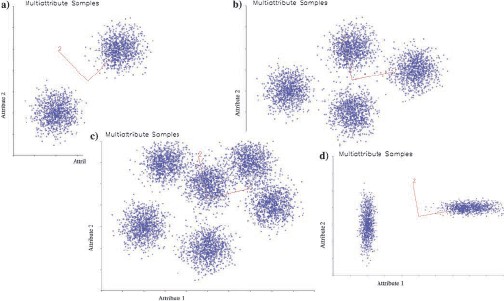
Several challenges and potential benefits of multiple attributes for interpretation are illustrated in Figure 1. Geologic features are revealed through attributes as coherent energy. When there is more than one attribute, we call these centers of coherent energy natural clusters. Identification and isolation of natural clusters are important parts of interpretation when working with multiple attributes. In Figure 1, we illustrate natural clusters in blue with 1000 samples of a Gaussian distribution in 2D. Figure 1a shows two natural clusters that project to either attribute scale (horizontal or vertical), so they would both be clearly visible in the seismic data, given a sufficient signal-to-noise ratio. Figure 1b shows four natural clusters that project to both attribute axes, but in this case, the horizontal attribute would see three clusters and would separate the left and right natural clusters clearly. The six natural clusters would be difficult to isolate in Figure 1c, and even the two natural clusters in Figure 1d, while clearly separated, have a special challenge. In Figure 1d, the right natural cluster is clearly separated and details could be resolved by attribute value. However, the left natural cluster would be separated by the attribute on the vertical axis and resolution cannot be as accurate because the higher values are obscured by projection from the right natural cluster. Based on the different 2D cluster examples in Figure 1a–1d, PCA has determined the largest variation in each example labeled one on the red lines and represents the first principal component. The second principal component is labeled two on the red lines.

Overview of principal component analysis

We illustrate PCA in 2D with the natural clusters of Figure 1, although the concepts extend to any dimension. Each dimension counts as an attribute. We first consider the two natural clusters in Figure 1a and find the centroid (average x and y points). We draw an axis through the point at some angle and project all the attribute points to the axis. Different angles will result in a different distribution of points on the axis. For an angle, there is a variance for all the distances from the centroid. PCA finds the angle that maximizes that variance (labeled one on red line). This direction is the first principal component, and this is called the first eigenvector.

The value of the variance is the first eigenvalue. Interestingly, there is an error for each data point that projects on the axis, and mathematically, the first principal component is also a least-squares fit to the data. If we subtract the least-squares fit, reducing the dimension by one, the second principal component (labeled two on red line) and second eigenvalue fit the residual. In Figure 1a, the first principal component passes through the centers of the natural clusters and the projection distribution is spread along the axis (the eigenvalue is 4.72). The first principal component is nearly equal parts of attribute one (50%) and attribute two (50%) because it lies nearly along a 45° line. We judge that both attributes are important and worth consideration.

The second principal component is perpendicular to the first, and the projections are restricted (eigenvalue is 0.22). Because the second principal component is so much smaller than the first (5%), we discard it. It is clear that the PCA alone reveals the importance of both attributes. In Figure 1b, the first principal component eigenvector is nearly horizontal. The x-component is 0.978, and the y-component is 0.208, so the first principal eigenvector is composed of 82% attribute one (horizontal axis) and 18% attribute two (vertical axis). The second component is 27% smaller than the first and is significant. In Figure 1c and 1d, the first principal components are also nearly horizontal with component mixes of 81%, 12% and 86%, 14%, respectively. The second components were 50% and 55%, respectively. We demonstrate PCA on these natural cluster models to illustrate that it is a valuable tool to evaluate the relative importance of attributes, although our data typically have many more natural clusters than attributes, and we must resort to automatic tools, such as SOM to hunt for natural clusters after a suitable suite of attributes has been selected.

Survey and attribute spaces

For this discussion, seismic data are represented by a 3D seismic survey data volume regularly sampled in location x or y and in time t or in depth Z. A 2D seismic line is treated as a 3D survey of one line. Each survey is represented by several attributes, f₁, f₂ … f_F. For example, the attributes might include the amplitude, Hilbert transform, envelope, phase, frequency, etc. As such, an individual sample x is represented in bold as an attribute vector of F-dimensions in survey space:

where ∈ reads “is a member of” and {..} is a set. Indices c, d, e, and f are indices of time or depth, trace, line number, and attribute, respectively. A sample drawn from the survey space with c, d, and e indices is a vector of attributes in a space R^F. It is important to note for later use that x does not change position in attribute space. The samples in a 3D survey drawn from X may lie in a fixed time or depth interval, a fixed interval offset from a horizon, or a variable interval between a pair of horizons. Moreover, samples may be restricted to a specific geographic area.

Normalization and covariance matrix

PCA starts with computation of the covariance matrix, which estimates the statistical correlation between pairs of attributes. Because the number range of an attribute is unconstrained, the mean and standard deviation of each attribute are computed and corresponding attribute samples are normalized by these two constants. In statistical calculations, these normalized attribute values are known as standard scores or Z scores. We note that the mean and standard deviation are often associated with a Gaussian distribution, but here we make no such assumption because it does not underlie all attributes. The phase attribute, for example, is often uniformly distributed across all angles, and envelopes are often lognormally distributed across amplitude values. However, standardization is a way to assure that all attributes are treated equally in the analyses to follow. Letting T stand for transpose, a multi-attribute sample on a single time or depth trace is represented as a column vector of F attributes:

where each component is a standardized attribute value and where the selected samples in the PCA analysis range from i = 1 to I. The covariance matrix is estimated by summing the dot product of pairs of multi-attribute samples over all I samples selected for the PCA analysis. That is, the covariance matrix

where the dot product is the matrix sum of the product x . x = xT x. The covariance matrix is symmetric, semipositive definite, and of dimension F × F.

Eigenvalues and eigenvectors

The PCA proceeds by computing the set of eigenvalues and eigenvectors for the covariance matrix. That is, for the covariance matrix, there are a set of F eigenvalues λ and eigenvectors v, which satisfy

This is a well-posed problem for which there are many stable numerical algorithms. For small F(<=10), the Jacobi method of diagonalization is convenient. For larger matrices, Householder transforms are used to reduce it to tridiagonal form, and then QR/QL deflation where Q, R, and L refer to parts of any matrix. Note that an eigenvector and eigenvalue are a matched pair. Eigenvectors are all orthogonal to each other and orthonormal when they are each of unit length. Mathematically, eigenvectors vi × vj = 0 for i ≠ j and vi × vj = 1 for i = j. The algorithms mentioned above compute orthonormal eigenvectors.

The list of eigenvalues is inspected to better understand how many attributes are important. The eigenvalue list that is sorted in decreasing order will be called the eigen-spectrum. We adopt the notation that the pair of eigenvalue and eigenvectors with the largest eigenvalue is {λ1V1}, and that the pair with the smallest eigenvalue is {λFVF}. A plot of the eigen-spectrum is drawn with a horizontal axis numbered one through F from left to right and a vertical axis that is increasing eigenvalue. For a multi-attribute seismic survey, a plot of the corresponding eigen-spectrum is often shaped like a decreasing exponential function. See Figure 3. The point where the eigen-spectrum generally flattens is particularly important. To the right of this point, additional eigenvalues are insignificant. Inspection of the eigen-spectrum constitutes the first and often the most important step in PCA (Figure 3b and 3c).

Unfortunately, eigenvalues reveal nothing about which attributes are important. On the other hand, simple identification of the number of attributes that are important is of considerable value. If L of F attributes are important, then F–L attributes are unimportant. Now, in general, seismic samples lie in an attribute space RF , but the PCA indicates that the data actually occupy a smaller space RL. The space RF−L is just noise.

The second step is to inspect eigenvectors. We proceed by picking the eigenvector corresponding to the largest eigenvalue fλ1v1g. This eigenvector, as a linear combination of attributes, points in the direction of maximum variance. The coefficients of the attribute components reveal the relative importance of the attributes. For example, suppose that there are four attributes of which two components are nearly zero and two are of equal value. We will conclude that for this eigenvector, we can identify two attributes that are important and two that are not. We find that a review of the eigenvectors for the first few eigenvalues of the eigen-spectrum reveal those attributes that are important in understanding the data (Figure 3b and 3c). Often the attributes of importance in this second stepmatch the number of significant attributes estimated in the first step.

Self-organizing maps

The self-organizing map (SOM) is a data visualization technique invented in 1982 by Kohonen (2001). This nonlinear approach reduces the dimensions of data through the use of unsupervised neural networks. SOM attempts to solve the issue that humans cannot visualize high-dimensional data. In other words, we cannot understand the relationship between numerous types of data all at once. SOM reduces dimensions by producing a 2D map that plots the similarities of the data by grouping similar data items together. Therefore, SOM analysis reduces dimensions and displays similarities. SOM approaches have been used in numerous fields, such as finance, industrial control, speech analysis, and astronomy (Fraser and Dickson, 2007). Roy et al. (2013) describe how neural networks have been used since the late 1990s in the industry to resolve various geoscience interpretation problems. In seismic interpretation, SOM is an ideal approach to understand how numerous seismic attributes relate and to classify various patterns in the data. Seismic data contain huge amounts of data samples, and they are highly continuous, greatly redundant, and significantly noisy (Coleou et al., 2003). The tremendous amount of samples from numerous seismic attributes exhibits significant organizational structure in the midst of noise. SOM analysis identifies these natural organizational structures in the form of clusters. These clusters reveal important information about the classification structure of natural groups that are difficult to view any other way. Dimensionality reduction properties of SOM are well known (Haykin, 2009). These natural groups and patterns in the data identified by the SOM analysis routinely reveal geologic features important in the interpretation process.

Overview of self-organizing maps

In a time or depth seismic survey, samples are first organized into multi-attribute samples, so all attributes are analyzed together as points. If there are F attributes, there are F numbers in each multi-attribute sample. SOM is a nonlinear mathematical process that introduces several new, empty multi-attribute samples called neurons.

These SOM neurons will hunt for natural clusters of energy in the seismic data. The neurons discussed in this article form a 2D mesh that will be illuminated in the data with a 2D color map.

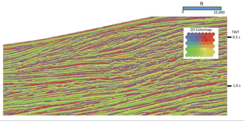
The SOM assigns initial values to the neurons, then for each multi-attribute sample, it finds the neuron closest to that sample by the Euclidean distance and advances it toward the sample by a small amount. Other neurons nearby in the mesh are also advanced. This process is repeated for each sample in the training set, thus completing one epoch of SOM learning. The extent of neuron movement during an epoch is an indicator of the level of SOM learning during that epoch. If an additional epoch is worthwhile, adjustments are made to the learning parameters and the next epoch is undertaken. When learning becomes insignificant, the process is complete. Figure 2 presents a portion of results of SOM learning on a 2D seismic line offshore of West Africa. For these results, a mesh of 8 × 8 neurons has six adjacent touching neurons. The 13 single-trace (instantaneous) attributes were selected for this analysis, so there was no communication between traces. These early results demonstrated that SOM learning was able to identify a great deal of geologic features. The 2D color map identifies different neurons with shades of green, blue, red, and yellow. The advantage of a 2D color map is that neurons that are adjacent to each other in the SOM analysis have similar shades of color. The figure reveals water-bottom reflections, shelf-edge peak and trough reflections, unconformities, onlaps/offlaps, and normal faults. These features are readily apparent on the SOM classification section, where amplitude is only one of 13 attributes used. Therefore, a SOM evaluation can incorporate several appropriate types of seismic attributes to define geology not easily interpreted from conventional seismic amplitude displays alone.

Self-organizing map neurons

Mathematically, a SOM neuron (loosely following notation by Haykin, 2009) lies in attribute space alongside the normalized data samples, which together lie in RF. Therefore, a neuron is also an F-dimensional column vector, noted here as w in bold. Neurons learn or adapt to the attribute data, but they also learn from each other. A neuron w lies in a mesh, which may be 1D, 2D, or 3D, and the connections between neurons are also specified. The neuron mesh is a topology of neuron connections in a neuron space. At this point in the discussion, the topology is unspecified, so we use a single subscript j as a place marker for counting neurons just as we use a single subscript i to count selected multi-attribute samples for SOM analysis.

A neuron learns by adjusting its position within attribute space as it is drawn toward nearby data samples. In general, the problem is to discover and identify an unknown number of natural clusters distributed in attribute space given the following: I data samples in survey space, F attributes in attribute space, and J neurons in neuron space. We are justified in searching for natural clusters because they are the multi-attribute seismic expression of seismic reflections, seismic facies, faults, and other geobodies, which we recognize in our data as geologic features. For example, faults are often identified by the single attribute of coherency. Flat spots are identified because they are flat. The AVO anomalies are identified as classes 1, 2, 2p, 3, or 4 by classifying several AVO attributes.

The number of multi-attribute samples is often in the millions, whereas the number of neurons is often in the dozens or hundreds. That is, the number of neurons J ≪ I. Were it not so, detection of natural clusters in attribute space would be hopeless. The task of a neural network is to assist us in our understanding of the data.

Neuron topology was first inspired by observation of the brain and other neural tissue. We present here results based on a neuron topology W, that is, 2D, so W lies in R2. Results shown in this paper have neuron meshes that are hexagonally connected (six adjacent points of contact).

Self-organizing-map learning

We now turn from a survey space perspective to an operational one to consider SOM learning as a process. SOM learning takes place during a series of time steps, but these time steps are not the familiar time steps of a seismic trace. Rather, these are time steps of learning. During SOM learning, neurons advance toward multi-attribute data samples, thus reducing error and thereby advancing learning. A SOM neuron adjusts itself by the following recursion:

where wj (n + 1) is the attribute position of neuron j at time step n. The recursion proceeds from time step n to n + 1. The update is in the direction toward xi along the “error” direction xi − wj (n). This is the direction that pulls the winning neuron toward the data sample. The amount of displacement is controlled by learning controls, η and h, which will be discussed shortly.

Equation 6 depends on w and x, so either select an x, and then use some strategy to select w, or vice versa. We elect to have all x participate in training, so we select x and use the following strategy to select w. The neuron nearest xi is the one for which the squared Euclidean distance,

is the smallest of all wj . This neuron is called the winning neuron, and this selection rule is central to a competitive learning strategy, which will be discussed shortly. For data sample xi, the resulting winning neuron will have subscript j, which results from scanning over all neurons with free subscript s under the minimum condition noted as

Now, the winning neuron for xi is found from

where the bar | reads “given” and the inverted A ∀ reads “for all.” That is, the winning neuron for data sample xi is wj . We observe that for every data sample, there is a winning neuron. One complete pass through all data samples fxi j i ¼ 1 to Ig is called one epoch. One epoch completes a single time step of learning. We typically exercise 60–100 epochs of training. It is noted that “epoch” as a unit of machine learning shares a sense of time with a geologic epoch, which is a division of time between periods and ages.

Returning to learning controls of equation 6, let the first term η change with time so as to be an adjustable learning rate control. We choose

with η0 as some initial learning rate and T2 as a learning decay factor. As time progresses, the learning control in equation 10 diminishes. This results in neurons that move large distances during early time steps move smaller distances in later time steps. The second term h of equation 6 is a little more complicated and calls into action the neuron topology W. Here, h is called the neighborhood function because it adjusts not only the winning neuron wj but also other neurons in the neighborhood of wj. Now, the neuron topology W is 2D, and the neighborhood function is given by

where d2J,K = [rj – rk] for a neuron at rj and the winning neuron at rk in the neuron topology. Distance d in equation 11 represents the distance between a winning neuron and another nearby neuron in neuron topology W. The neighborhood function in equation 11depends on the distance between a neuron and the winning neuron and also time. The time-varying part of equation 11 is defined as

where σ0 is the initial neighborhood distance and τ1 is the neighborhood decay factor. As σ increases with time, h decreases with time. We define an edge of the neighborhood as the distance beyond which the neuron weight is negligible and treated as zero. In 2D neuron topologies, the neighborhood edge is defined by a radius. Let this cut-off distance depend on a free constant ζ. In equation 11, we set h = ζ and solve for dmax as

The neighborhood edge distance dmax → 0 as ζ → 0. As time marches on, the neighborhood edge shrinks to zero and continued processing steps of SOM are similar to K-means clustering (Bishop, 2007). Additional details of SOM learning are found in Appendix A on SOM analysis operation.

Harvesting

Rather than apply the SOM learning process to a large time or depth window spanning an entire 3D survey, we sample a subset of the full complement of multi-attribute samples in a process called harvesting. This is first introduced by Taner et al. (2009) and is described in more detail by Smith and Taner (2010).

First, a representative set of harvest patches from the 3D survey is selected, and then on each of these patches, we conduct independent SOM training. Each harvest patch is one or more lines, and each SOM analysis yields a set of winning neurons. We then apply a harvest rule to select the set of winning neurons that best represent the full set of data samples of interest.

A variety of harvest rules has been investigated. We often choose a harvest rule based on best learning. Best learning selects the winning neuron set for the SOM training, in which there has been the largest proportional reduction of error between initial and final epochs on the data that were presented. The error is measured by summing distances as a measure of how near the winning neurons are to their respective data samples. The largest reduction in error is the indicator of best learning. Additional details on harvest sampling and harvest rules are found in Appendix A on SOM analysis operation.

Self-organizing-map classification and probabilities

Once natural clusters have been identified, it is a simple task to classify samples in survey space as members of a particular cluster. That is, once the learning process has completed, the winning neuron set is used to classify each selected multi-attribute sample in the survey. Each neuron in the winning neuron set (j = 1 to J) is tested with equation 9 against each selected sample in the survey (i = 1 to I). Each selected sample then has assigned to it a neuron that is nearest to that sample in Euclidean distance. The winning neuron index is assigned to that sample in the survey.

Every sample in the survey has associated with it a winning neuron separated by a Euclidean distance that is the square root of equation 7. After classification, we study the Euclidean distances to see how well the neurons fit. Although there are perhaps many millions of survey samples, there are far fewer neurons, so for each neuron, we collect its distribution of survey sample distances. Some samples near the neuron are a good fit, and some samples far from the neuron are a poor fit. We quantify the goodness-of-fit by distance variance as described in Appendix A. Certainly, the probability of a correct classification of a neuron to a data sample is higher when the distance is smaller than when it is larger. So, in addition to assigning a winning neuron index to a sample, we also assign a classification probability. The classification probability ranges from one to zero corresponding to distance separations of zero to infinity. Those areas in the survey where the classification probability is low correspond to areas where no neuron fits the data very well. In other words, anomalous regions in the survey are noted by low probability. Additional comments are found in Appendix A.

Case Studies – Offshore Gulf of Mexico

This case study is located offshore Louisiana in the Gulf of Mexico in a water depth of 143 m (470 ft). This shallow field (approximately 1188 m [3900 ft]) has two producing wells that were drilled on the upthrown side of an east–west-trending normal fault and into an amplitude anomaly identified on the available 3D seismic data. The normally pressured reservoir is approximately 30 m (100 ft) thick and located in a typical “bright-spot” setting, i.e., a Class 3 AVO geologic setting (Rutherford and Williams, 1989). The goal of the multi-attribute analysis is to more clearly identify possible DHI characteristics such as flat spots (hydrocarbon contacts) and attenuation effects to better understand the existing reservoir and provide important approaches to decrease risk for future exploration in the area.

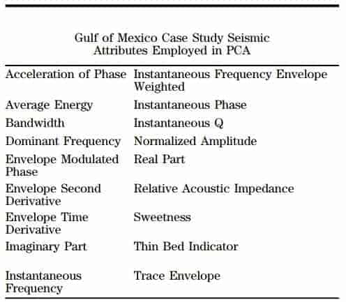
Initially, 18 instantaneous seismic attributes were generated from the 3D data in this area (see Table 2). These seismic attributes were put into a PCA evaluation to determine which produced the largest variation in the data and the most meaningful attributes for SOM analysis. The PCA was computed in a window 20 ms above and 150 ms below the mapped top of the reservoir over the entire survey, which encompassed approximately 26 km2 (10 mi2). Figure 3a displays a chart with each bar representing the highest eigenvalue on its associated inline over the displayed portion of the survey. The bars in red in Figure 3a specifically denote the inlines that cover the areal extent of the amplitude feature and the average of their eigenvalue results are displayed in Figure 3b and 3c. Figure 3b displays the principal components from the selected inlines over the anomalous feature with the highest eigenvalue (first principal component) indicating the percentage of seismic attributes contributing to this largest variation in the data. In this first principal component, the top seismic attributes include the envelope, envelope modulated phase, envelope second derivative, sweetness, and average energy, all of which account for more than 63% of the variance of all the instantaneous attributes in this PCA evaluation. Figure 3c displays the PCA results, but this time the second highest eigenvalue was selected and produced a different set of seismic attributes. The top seismic attributes from the second principal component include instantaneous frequency, thin bed indicator, acceleration of phase, and dominant frequency, which total almost 70% of the variance of the 18 instantaneous seismic attributes analyzed. These results suggest that when applied to an SOM analysis, perhaps the two sets of seismic attributes for the first and second principal components will help to define two different types of anomalous features or different characteristics of the same feature.

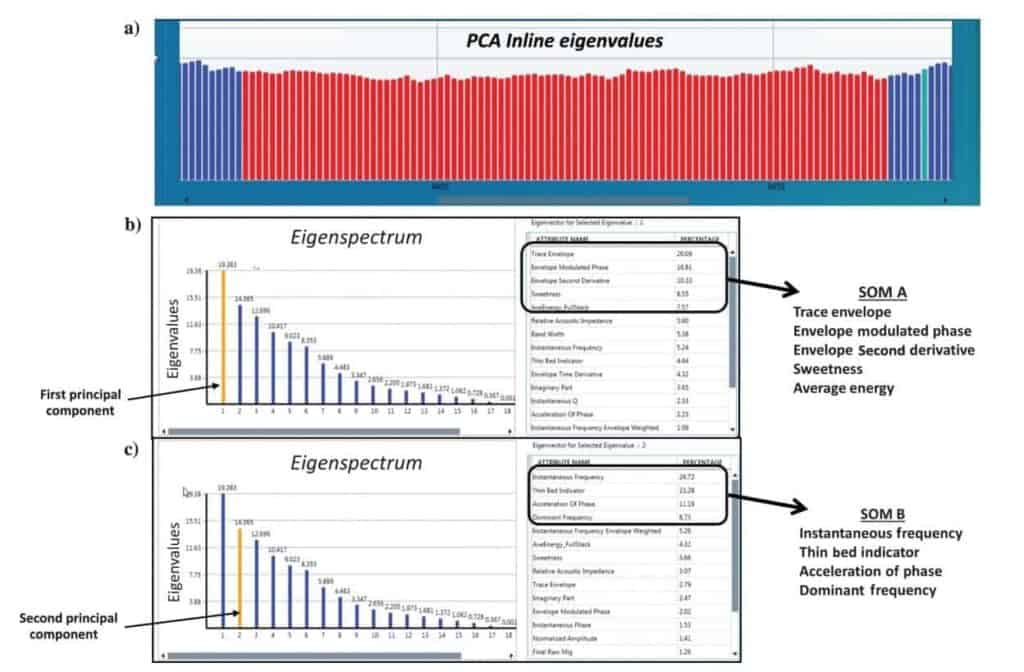
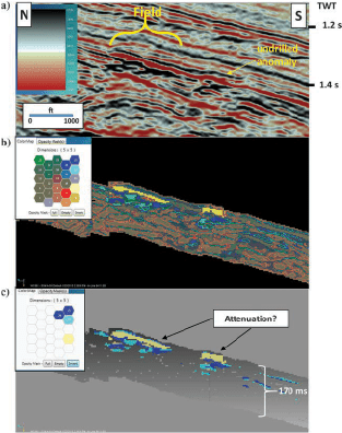
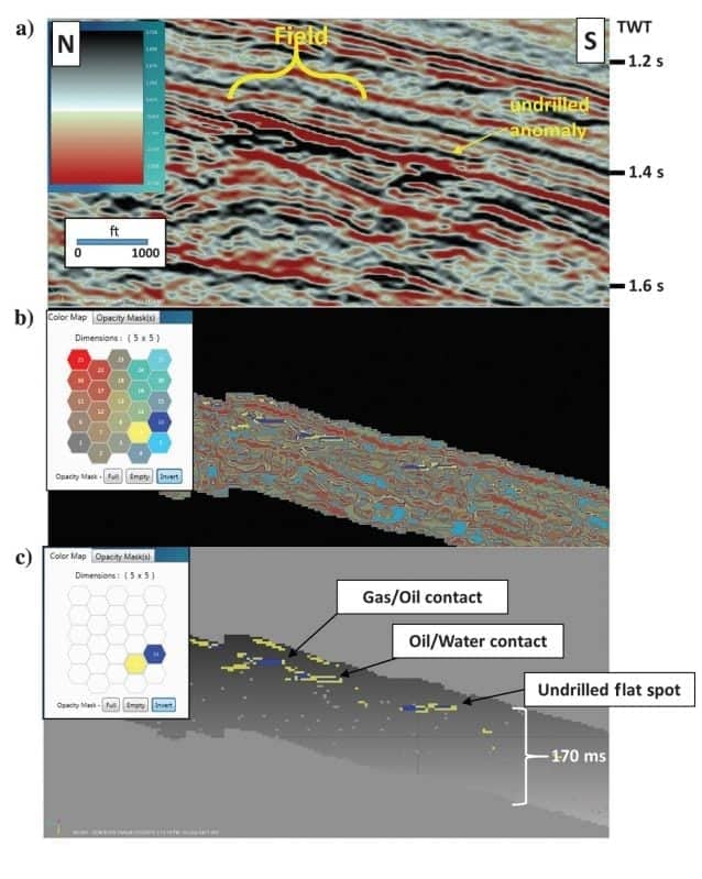
The first SOM analysis (SOM A) incorporates the seismic attributes defined by the PCA with the highest variation in the data, i.e., the five highest percentage contributing attributes in Figure 3b. Several neuron counts for SOM analyses were run on the data with lower count matrices revealing broad, discrete features and the higher counts displaying more detail and less variation. The SOM results from a 5 × 5 matrix of neurons (25) were selected for this paper. The north–south line through the field in Figures 4 and 5 shows the original stacked amplitude data and classification results from the SOM analyses. In Figure 4b, the color map associated with the SOM classification results indicates all 25 neurons are displayed, and Figure 4c shows results with four interpreted neurons highlighted. Based on the location of the hydrocarbons determined from well control, it is interpreted from the SOM results that attenuation in the reservoir is very pronounced with this evaluation. As Figure 4b and 4c reveal, there is apparent absorption banding in the reservoir above the known hydrocarbon contacts defined by the wells in the field. This makes sense because the seismic attributes used are sensitive to relatively low-frequency broad variations in the seismic signal often associated with attenuation effects. This combination of seismic attributes used in the SOM analysis generates a more pronounced and clearer picture of attenuation in the reservoir than any one of the seismic attributes or the original amplitude volume individually. Downdip of the field is another undrilled anomaly that also reveals apparent attenuation effects.

The second SOM evaluation (SOM B) includes the seismic attributes with the highest percentages from the second principal component based on the PCA (see Figure 3). It is important to note that these attributes are different than the attributes determined from the first principal component. With a 5 × 5 neuron matrix, Figure 5 shows the classification results from this SOM evaluation on the same north–south line as Figure 4, and it clearly identifies several hydrocarbon contacts in the form of flat spots. These hydrocarbon contacts in the field are confirmed by the well control. Figure 5b defines three apparent flat spots, which are further isolated in Figure 5c that displays these features with two neurons. The gas/oil contact in the field was very difficult to see on the original seismic data, but it is well defined and mappable from this SOM analysis. The oil/water contact in the field is represented by a flat spot that defines the overall base of the hydrocarbon reservoir. Hints of this oil/water contact were interpreted from the original amplitude data, but the second SOM classification provides important information to clearly define the areal extent of reservoir. Downdip of the field is another apparent flat spot event that is undrilled and is similar to the flat spots identified in the field. Based on SOM evaluations A and B in the field that reveal similar known attenuation and flat spot results, respectively, there is a high probability this undrilled feature contains hydrocarbons.

Shallow Yegua trend in Gulf Coast of Texas

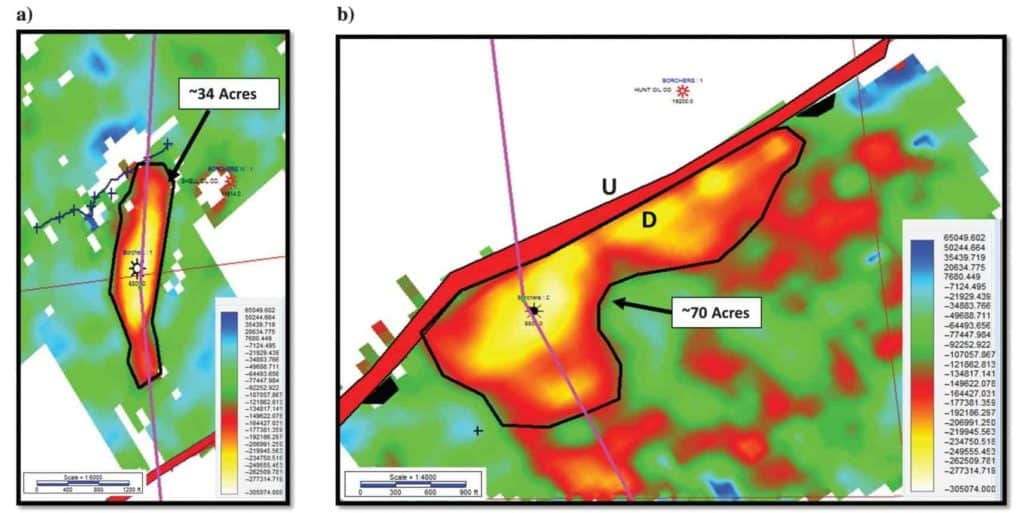
This case study is located in Lavaca County, Texas, and targets the Yegua Formation at approximately 1828 m (6000 ft). The initial well was drilled just downthrown on a small southwest–northeast regional fault, with a subsequent well being drilled on the upthrown side. There were small stacked data amplitude anomalies on the available 3D seismic data at both well locations. The Yegua in the wells is approximately 5 m (18 ft) thick and is composed of thinly laminated sands. Porosities range from 24% to 30% and are normally pressured. Because of the thin laminations and often lower porosities, these anomalies exhibit a class 2 AVO response, with near-zero amplitudes on the near offsets and an increase in negative amplitude with offset (Rutherford and Williams, 1989). The goal of the multi-attribute analysis was to determine the full extent of the reservoir because both wells were performing much better than the size of the amplitude anomaly indicated from the stacked seismic data (Figure 6a and 6b). The first well drilled downthrown had a stacked data amplitude anomaly of approximately 70 acres, whereas the second well upthrown had an anomaly of about 34 acres.

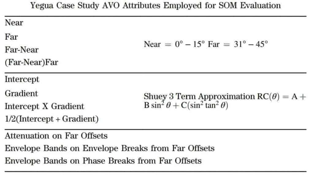
The gathers that came with the seismic data had been conditioned and were used in creating very specific AVO volumes conducive to the identification of class 2 AVO anomalies in this geologic setting. In this case, the AVO attributes selected were based on the interpreter’s experience in this geologic setting.

Table 3 lists the AVO attributes and the attributes generated from the AVO attributes used in this SOM evaluation. The intercept and gradient volumes were created using the Shuey three-term approximation of the Zoeppritz equation (Shuey, 1985). The near-offset volume was produced from the

0°–15° offsets and the far-offset volume from the 31°–45° offsets. The attenuation, envelope bands on the envelope breaks, and envelope bands on the phase breaks seismic attributes were all calculated from the far-offset volume. For this SOM evaluation, an 8 × 8 matrix (64 neurons) was used.

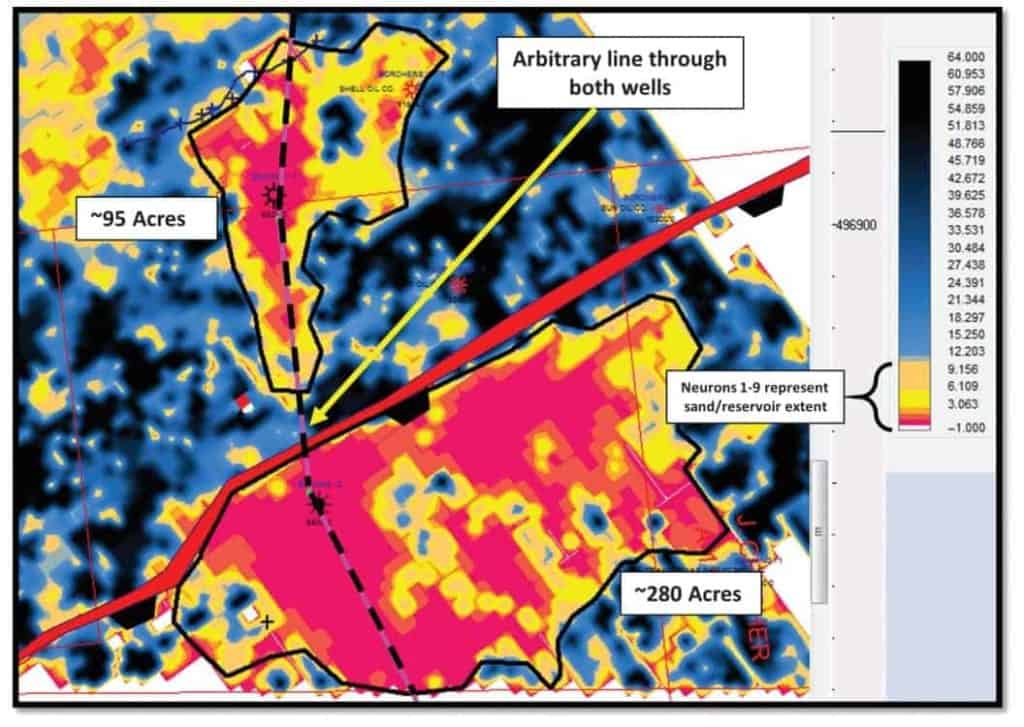
Figure 7 displays the areal distribution of the SOM classification at the Yegua interval. The interpretation of this SOM classification is that the two areas outlined represent the hydrocarbon producing portion of the reservoir and all the connectivity of the sand feeding into the well bores. On the downthrown side of the fault, the drainage area has increased to approximately 280 acres, which supports the engineering and pressure data. The areal extent of the drainage area on the upthrown reservoir has increased to approximately 95 acres, and again agreeing with the production data. It is apparent that the upthrown well is in the feeder channel, which deposited sand across the then-active fault and splays along the fault scarp.

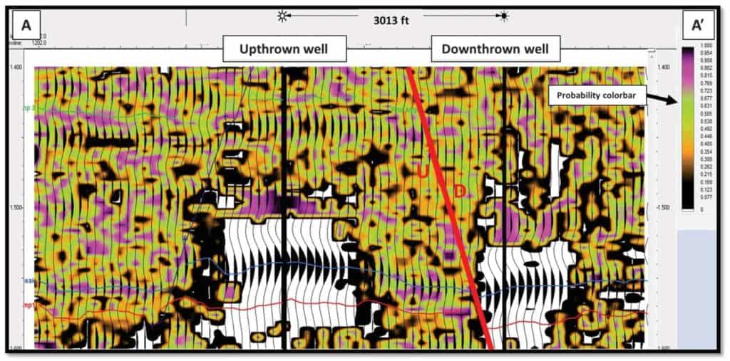
In addition to the SOM classification, the anomalous character of these sands can be easily seen in the probability results from the SOM analysis (Figure 8). The probability is a measure of how far the neuron is from its identified cluster (see Appendix A). The low-probability zones denote the most anomalous areas determined from the SOM evaluation. The most anomalous areas typically will have the lowest probability, whereas the events that are present over most of the data, such as horizons, interfaces, etc., will have higher probabilities. Because the seismic attributes that went into this SOM analysis are AVO-related attributes that enhance DHI features, these low-probability zones are interpreted to be associated with the Yegua hydrocarbonbearing sands.

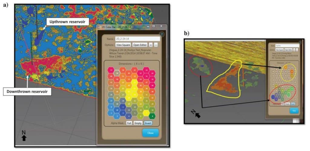
Figure 9 displays the SOM classification results with a time slice located at the base of the upthrown reservoir and the upper portion of the downthrown reservoir. There is a slight dip component in the figure. Figure 9a reveals the total SOM classification results with all 64 neurons as indicated by the associated 2D color map. Figure 9b is the same time slice slightly rotated to the west with very specific neurons highlighted in the 2D color map defining the upthrown and downthrown fields. The advantage of SOM classification analyses is the ability to isolate specific neurons that highlight desired geologic features. In this case, the SOM classification of the AVO-related attributes was able to define the reservoirs drilled by each of the wells and provide a more accurate picture of their areal distributions than the stacked data amplitude information.

Eagle Ford Shale

This study is conducted using 3D seismic data from the Eagle Ford Shale resource play of south Texas. Understanding the existing fault and fracture patterns in the Eagle Ford Shale is critical to optimizing well locations, well plans, and fracture treatment design. To identify fracture trends, the industry routinely uses various seismic techniques, such as processing of seismic attributes, especially geometric attributes, to derive the maximum structural information from the data.

Geometric seismic attributes describe the spatial and temporal relationship of all other attributes (Taner, 2003). The two main categories of these multitrace attributes are coherency/similarity and curvature. The objective of coherency/similarity attributes is to enhance the visibility of the geometric characteristics of seismic data such as dip, azimuth, and continuity. Curvature is a measure of how bent or deformed a surface is at a particular point with the more deformed the surface the more the curvature. These characteristics measure the lateral relationships in the data and emphasize the continuity of events such as faults, fractures, and folds.

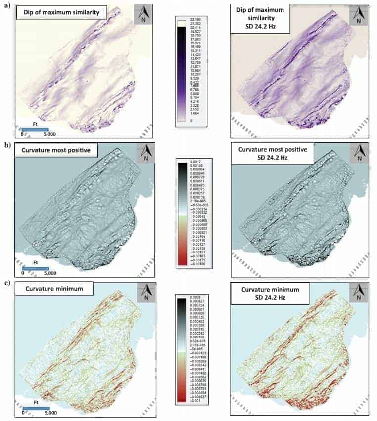
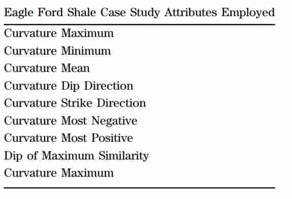
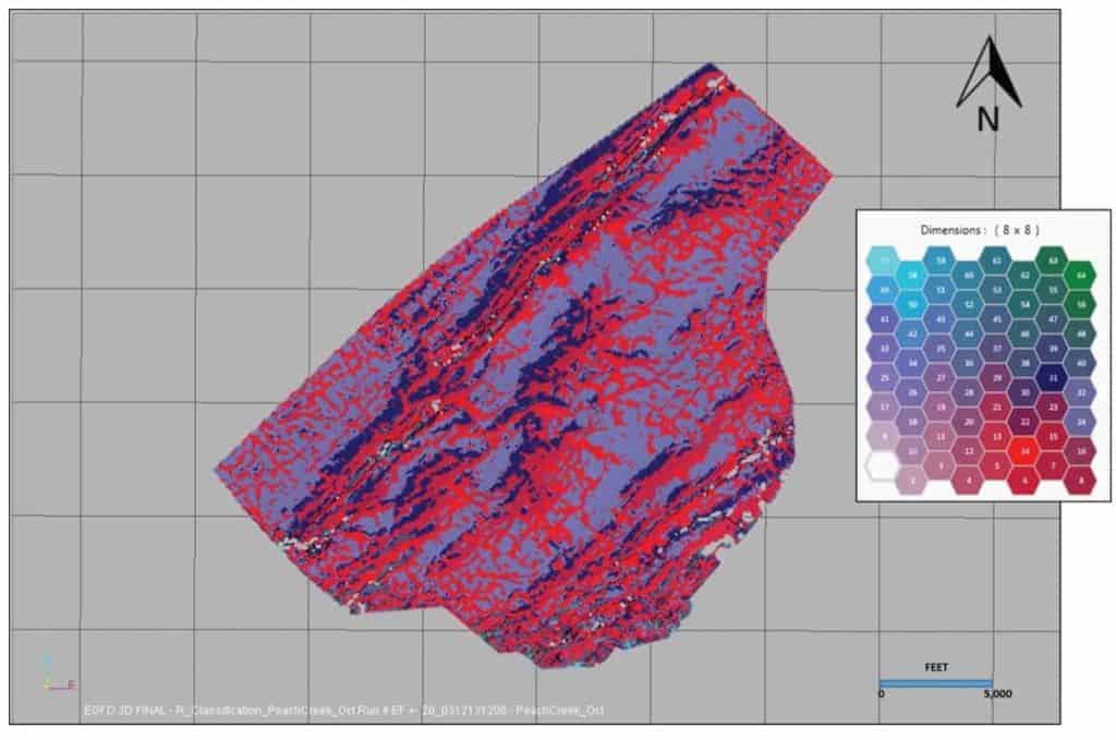
The goal of this case study is to more accurately define the fault and fracture patterns (regional stress fields) than what had already been revealed in running geometric attributes over the existing stacked seismic data. Initially, 18 instantaneous attributes, 14 coherency/similarity attributes, 10 curvature attributes, and 40 frequency subband volumes of spectral decomposition were generated. In the evaluation of these seismic attributes, it was determined in the Eagle Ford interval that the highest energy resided in the 22- to 26-Hz range. Therefore, a comparison was made with geometric attributes computed from a spectral decomposition volume with a center frequency of 24.2 Hz with the same geometric attributes computed from the original fullfrequency volume. At the Eagle Ford interval, Figure 10 compares three geometric attributes generated from the original seismic volume with the same geometric attributes generated from the 24.2-Hz spectral decomposition volume. It is evident from each of these geometric attributes that there is an improvement in the image delineation of fault/fracture trends with the spectral decomposition volumes. Based on the results of the geometric attributes produced from the 24.2-Hz volume and trends in the associated PCA interpretation, Table 4 lists the attributes used in the SOM analysis over the Eagle Ford interval. This SOM analysis incorporated an 8 × 8 matrix (64 neurons). Figure 11 displays the results at the top of the Eagle Ford Shale of the SOM analysis using the nine geometric attributes computed from the 24.2-Hz spectral decomposition volume. The associated 2D color map in Figure 11 provides the correlation of colors to neurons. There are very clear northeast–southwest trends of relatively large fault and fracture systems, which are typical for the Eagle Ford Shale (primarily in dark blue). What is also evident is an orthogonal set of events running southeast–northwest and east–west (red).

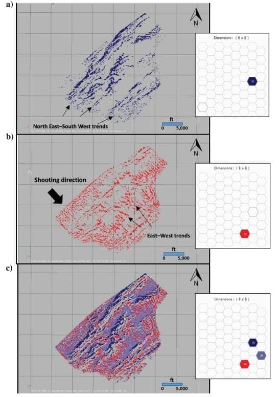
To further evaluate the SOM results, individual clusters or patterns in the data are isolated with the highlighting of specific neurons in the 2D color map in Figure 12. Figure 12a indicates neuron 31 (blue) is defining the larger northeast–southwest fault/fracture trends in the Eagle Ford Shale. Figure 12b with neuron 14 (red) indicates orthogonal sets of events. Because the survey was acquired southeast–northwest, it could be interpreted that the similar trending events in Figure 12b are possible acquisition footprint effects, but there are very clear indications of east–west lineations also. These east–west lineations probably represent fault/fracture trends orthogonal to the major northeast–southwest trends in the region. Figure 12c displays the neurons from Figure 12a and 12b, as well as neuron 24 (dark gray). With these three neurons highlighted, it is easy to see the fault and fracture trends against a background, where neuron 24 displays a relatively smooth and nonfaulted region. The key issue in this evaluation is that the SOM analysis allows the breakout of the fault/fracture trends and allows the geoscientist tomake better informed decisions in their interpretation.

Conclusions

Seismic attributes, which are any measurable properties of seismic data, aid interpreters in identifying geologic features, which are not clearly understood in the original data. However, the enormous amount of information generated from seismic attributes and the difficulty in understanding how these attributes when combined define geology, requires another approach in the interpretation workflow. The application of PCA can help interpreters to identify seismic attributes that show the most variance in the data for a given geologic setting. The PCA works very well in geologic settings, where anomalous features stand out from the background data, such as class 3 AVO settings that exhibit DHI characteristics. The PCA helps to determine, which attributes to use in a multi-attribute analysis using SOMs.

Applying current computing technology, visualization techniques, and understanding of appropriate parameters for SOM, enables interpreters to take multiple seismic attributes and identify the natural organizational patterns in the data. Multiple-attribute analyses are beneficial when single attributes are indistinct. These natural patterns or clusters represent geologic information embedded in the data and can help to identify geologic features, geobodies, and aspects of geology that often cannot be interpreted by any other means. The SOM evaluations have proven to be beneficial in essentially all geologic settings including unconventional resource plays, moderately compacted onshore regions, and offshore unconsolidated sediments. An important observation in the three case studies is that the seismic attributes used in each SOM analysis were different. This indicates the appropriate seismic attributes to use in any SOM evaluation should be based on the interpretation problem to be solved and the associated geologic setting. The application of PCA and SOM can not only identify geologic patterns not seen previously in the seismic data, but it also can increase or decrease confidence in already interpreted features. In other words, this multi-attribute approach provides a methodology to produce a more accurate risk assessment of a geoscientist’s interpretation and may represent the next generation of advanced interpretation.

References

Abele, S., and R. Roden, 2012, Fracture detection interpretation beyond conventional seismic approaches: Presented at AAPG Eastern Section Meeting, Poster AAPG-ICE.
Balch, A. H., 1971, Color sonograms: A new dimension in seismic data interpretation: Geophysics, 36, 1074–1098.
Barnes, A., 2006, Too many seismic attributes?: CSEG Recorder, 31, 41–45.
Bishop, C. M., 2006, Pattern recognition and machine learning: Springer, 561–565.
Bishop, C. M., 2007, Neural networks for pattern recognition: Oxford, 240–245.
Bishop, C. M., M. Svensen, and C. K. I. Williams, 1998, GTM: The generative topographic mapping: Neural Computation, 10, 215–234.
Brown, A. R., 1996, Interpretation of three-dimensional seismic data, 3rd ed.: AAPG Memoir 42.
Chen, Q., and S. Sidney, 1997, Seismic attribute technology for reservoir forecasting and monitoring: The Leading Edge, 16, 445–448.
Chopra, S., and K. Marfurt, 2007, Seismic attributes for prospect identification and reservoir characterization, SEG, Geophysical Development Series.
Coleou, T., M. Poupon, and A. Kostia, 2003, Unsupervised seismic facies classification: A review and comparison of techniques and implementation: The Leading Edge, 22, 942–953.
Erwin, E., K. Obermayer, and K. Schulten, 1992, Self-organizing maps: Ordering, convergence properties and energy functions: Biological Cybernetics, 67, 47–55.
Fraser, S. H., and B. L. Dickson, 2007, A new method of data integration and integrated data interpretation: Self-organizing maps, in B. Milkereit, ed., Proceedings of Exploration 07: Fifth Decennial International Conference on Mineral Exploration, 907–910.
Guo, H., K. J. Marfurt, and J. Liu, 2009, Principal component spectral analysis: Geophysics, 74, no. 4, P35–P43.
Haykin, S., 2009, Neural networks and learning machines, 3rd ed.: Pearson.
Kalkomey, C. T., 1997, Potential risks when using seismic attributes as predictors of reservoir properties: The Leading Edge, 16, 247–251.
Kohonen, T., 2001, Self organizing maps: Third extended edition, Springer, Series in Information Services.
Liner, C., 1999, Elements of 3-D seismology: PennWell.
Roy, A., B. L. Dowdell, and K. J. Marfurt, 2013, Characterizing a Mississippian tripolitic chert reservoir using 3D unsupervised and supervised multi-attribute seismic facies analysis: An example from Osage County, Oklahoma: Interpretation, 1, no. 2, SB109–SB124.
Rutherford, S. R., and R. H. Williams, 1989, Amplitude-versus-offset variations in gas sands: Geophysics, 54, 680–688.
Schlumberger Oilfield Glossary, 2015, online reference, http://www.glossary.oilfield.slb.com.
Shuey, R. T., 1985, A simplification of the Zoeppritz equations: Geophysics, 50, 609–614.
Smith, T., and M. T. Taner, 2010, Natural clusters in multiattribute seismics found with self-organizing maps: Source and signal processing section paper 5: Presented at Robinson-Treitel Spring Symposium by GSH/SEG, Extended Abstracts.
Taner, M. T., 2003, Attributes revisited, https://www.rocksolidimages.com/attributes-revisited, accessed 13 August 2013.
Taner, M. T., F. Koehler, and R. E. Sheriff, 1979, Complex seismic trace analysis: Geophysics, 44, 1041–1063.
Taner, M. T., and R. E. Sheriff, 1977, Application of amplitude, frequency, and other attributes, to stratigraphic and hydrocarbon determination, in C. E. Payton, ed., Applications to hydrocarbon exploration: AAPG Memoir 26, 301–327.
Taner, M. T., S. Treitel, and T. Smith, 2009, Self-organizing maps of multi-attribute 3D seismic reflection surveys, Presented at the 79th International SEG Convention, SEG 2009 Workshop on “What’s New in Seismic Interpretation,” Paper no. 6.