Tom Smith, Geophysical Insights and Sven Treitel, TriDekon | November 2015
Self-Organizing Neural Nets for Automatic Anomaly Identification
Self-organizing maps are a practical way to identify natural clusters in multi-attribute seismic data. Curvature measure identifies neurons that have found natural clusters from those that have not. Harvesting is a methodology for measuring consistency and delivering the most consistent classification. Those portions of the classification with low probability are an indicator of multi-attribute anomalies which warrant further investigation.
Introduction
Over the past several years, the growth in seismic data volumes has multiplied many times. Often a prospect is evaluated with a primary 3D survey along with 5 to 25 attributes which serve both general and unique purposes. These are well laid out by Chopra and Marfurt, 2007. Self-organizing maps (Kohonen, 2001), or SOM for short, are a type of unsupervised neural network which fit themselves to the pattern of information in multi-dimensional data in an orderly fashion.
Multi-attributes and natural clusters
We organize a 3D seismic survey data volume regularly sampled in location X, Y and time T (or depth estimate Z). Each survey sample is represented by a number of attributes, f1, f2, …, fF. An individual sample is represented in bold as a vector with four subscripts. Together, they represent the survey space k , so the set of samples
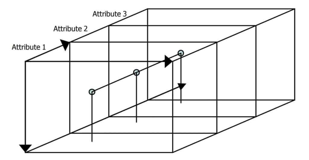
with indices c, d, e and f represent time, trace, line number and attribute number, respectively. It is convenient to represent a sample fixed in space as a vector of F attributes in attribute space. Let this set of attribute samples {x1, x2,…xi,…, xI} be taken from k and range from 1 to I. The layout of survey space representing a 3D attribute space is illustrated in Figure 1. An attribute sample, marked as resting on the top of pins, consists of a vector of three attribute values at a fixed location.
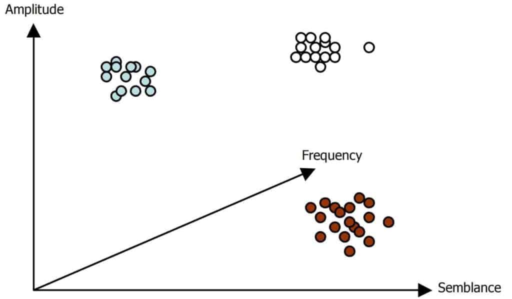
The sample of Figure 1 resides in attribute space as shown in Figure 2. Included in the illustration are other samples with similar properties. These natural clusters are regions of higher density which can constitute various seismic events with varying attribute characteristics. A natural cluster would register as a maximum in a probability distribution function. However, a large number of attributes entails a histogram of impractically high dimensionality.
Self-Organizing Map (SOM)
A SOM neuron lies in attribute space alongside the data samples. Therefore, a neuron is also an F-dimensional vector noted here as w in bold. The neuron w lies in a topology j called the neuron space. At this point in the discussion, the topology is unspecified so use a single subscript t as a place marker for any number of dimensions. Whereas data samples remain fixed in attribute space,
neurons are allowed to move freely in attribute space. They are then progressively drawn toward the data samples.
A neuron “learns” by adjusting its position within the attribute space as it is drawn toward nearby data points. Then let us define a self-organizing neural network as a collection of neurons {w1, w2,…, wi,…, wJ} with an index ranging from 1 through J. The neural network learns as its neurons adjust to natural clusters in attribute space. In general the problem is to discover and identify an unknown number of natural clusters distributed in attribute space, given the following information: I data samples in survey space; F attributes in attribute space; and J neurons in neuron space. The SOM was invented by T. Kohonen and discussed in Kohonen, T., 2001. It addresses such issues as a classic problem in statistical classification.
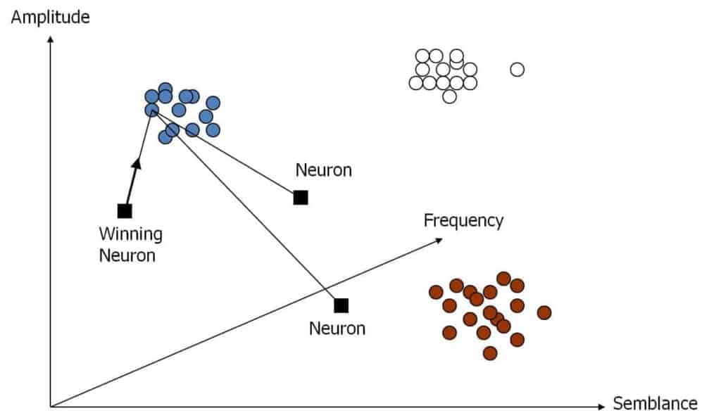
In Figure 3 we place three neurons at arbitrary locations in attribute space from Figure 2. A simple process of learning proceeds as follows. Given the first sample, one computes the distance from the data sample to each of the 3 neurons and selects the closest one. We choose the Euclidean distance as our measure of distance.
The winning neuron with subscript k is defined
where j ranges over all neurons. In Figure 3, the neuron on the left is identified as the winning neuron. The winning neuron advances toward the data sample along a vector which is a fraction of the distance from the data sample. Then the second sample is selected and the process is repeated. In this example, the neuron marked as the winning neuron may end up in the leftmost cluster of the Figure. The lowermost neuron may end up near the center of the lowermost cluster on the right and the third neuron might end up in the cluster in the upper right of the Figure. This type of learning is called competitive because only the winning neuron moves toward the data.
A key point to note is that after one complete pass through the data samples, although not every neuron may have moved toward any data points, nevertheless every sample has one and only one winning neuron. A complete pass through the data is called an epoch. Many epochs may be required before the neurons have completed their clustering task.
The process just described is the basis of the SOM. A SOM neuron adjusts itself by the following recursion.
where wj(n) is the attribute position of neuron j at time step n and k is the winning neuron number. The recursion proceeds from time step n to step n + 1. The update is in the direction toward x along the “error” direction x–wj(n). The amount of displacement is controlled by the learning control parameters, η and h, which are both scalars.
The η term grows smaller with each time step, so large neuron adjustments during early epochs smoothly taper to smaller adjustments later.
The h term embodies still another type of learning and which is also part of the SOM learning process.
Here d is the Euclidean distance between neurons in the neuron space introduced in equation (2)
And
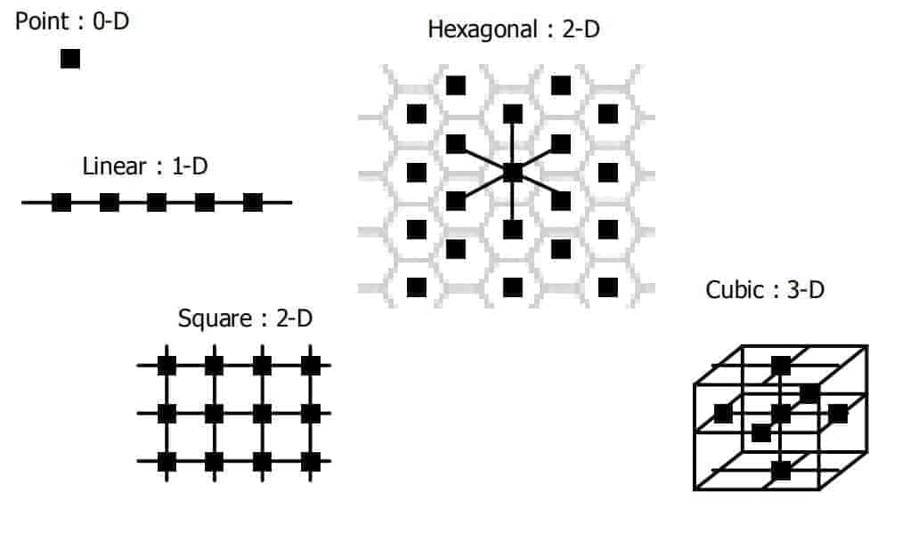
In equation (7), y is a positional vector in the neuron topology. Several options for neuron topology in neuron space are shown in Figure 4.
From equation (6) we observe that not only is the winning neuron moving toward a data point, other neurons around the winning neuron are moving as well. These neurons constitute the winning neuron neighborhood.
In the hexagonal topology of Figure 4, note that the marked neuron has 6 nearest neighbors. If this neuron is selected as a winning neuron, equations (6) and (7) indicate that the 6 nearest neurons move toward the data sample by a like amount. More distant neurons from the winning neuron move a lesser amount.
Neighborhoods of neuron movement constitute cooperative learning. For a 2D neuron space, hexagonal topology offers the maximum number of similarly distant neurons. Here we have chosen a hexagonal neural network because it maximizes cooperative learning in 2D. The SOM embodies both competitive and cooperative learning rules (Haykin, 2009).
Curvature measure
To search for natural clusters and to avoid the curse of dimensionality (Bishop, 2007), we allow the SOM to find them for us. However, there is no assurance that at the end of such a SOM analysis the neurons have come to rest at or near the centers of natural clusters. To address this issue, we turn to the simple definition of a maximum. A natural cluster is by definition a denser region of attribute space. It is identified as a maximum in a probability distribution function through analysis of a histogram. In 1D the histogram has a maximum; in 2D the histogram is a maximum in 2 orthogonal directions and so on.
In F-dimensional attribute space, a natural cluster is revealed by a peak in the probability distribution function of all F attributes. Recall that at the end of an epoch there is a one-to-one relationship between a data sample and its winning neuron. That implies that to every winning neuron there corresponds a set of one or more data samples.
Then for some winning neuron with index k, there exists a set of data samples x for which
and where k N include the samples drawn from k for that winning neuron. Some winning neurons in equation (9) have a small collection of x samples while others will have a larger collection.
In the set x for a winning neuron wk, for each of the f attributes [1 to F] we can determine a histogram. If there is a peak in the histogram we have found a higher magnitude in the probability distribution in that particular dimension and so score this attribute as a success. We count all attributes in this way (1 for success or 0 for failure) and divide the result by the number of attributes. Curvature measures density and lies in the range [0,1]. Each neuron and each attribute has a curvature measure.
Harvesting and consistency
A harvesting process consists of three steps. First, unsupervised neural network analyses are run on independent sets of data that have been drawn from a 2D or
3D survey. A rule is then used to decide which candidate is the best solution. Finally, the set of neurons of the best solution are used to classify the entire survey.
We have conducted a series of SOM analysis and classification steps for the Stratton Field 3D Seismic Survey (provided to us by courtesy of the Bureau of Economic Geology and the University of Texas). A time window of 1.2 to 1.8s was selected for SOM analysis with an 8 x 8 hexagonal network and 100 learning epochs. We measured performance by standard deviation of error between data samples and their winning neurons. Standard deviation error reduction was typically 35%. A separate SOM analysis was conducted on each of the 100 lines in order to assess consistency of results. The SOM results were highly consistent with a variation of final standard deviation of error of only 1.5% of the mean. The rule used here is to select the SOM solution for the line which best fits its data through smallest error of fit.
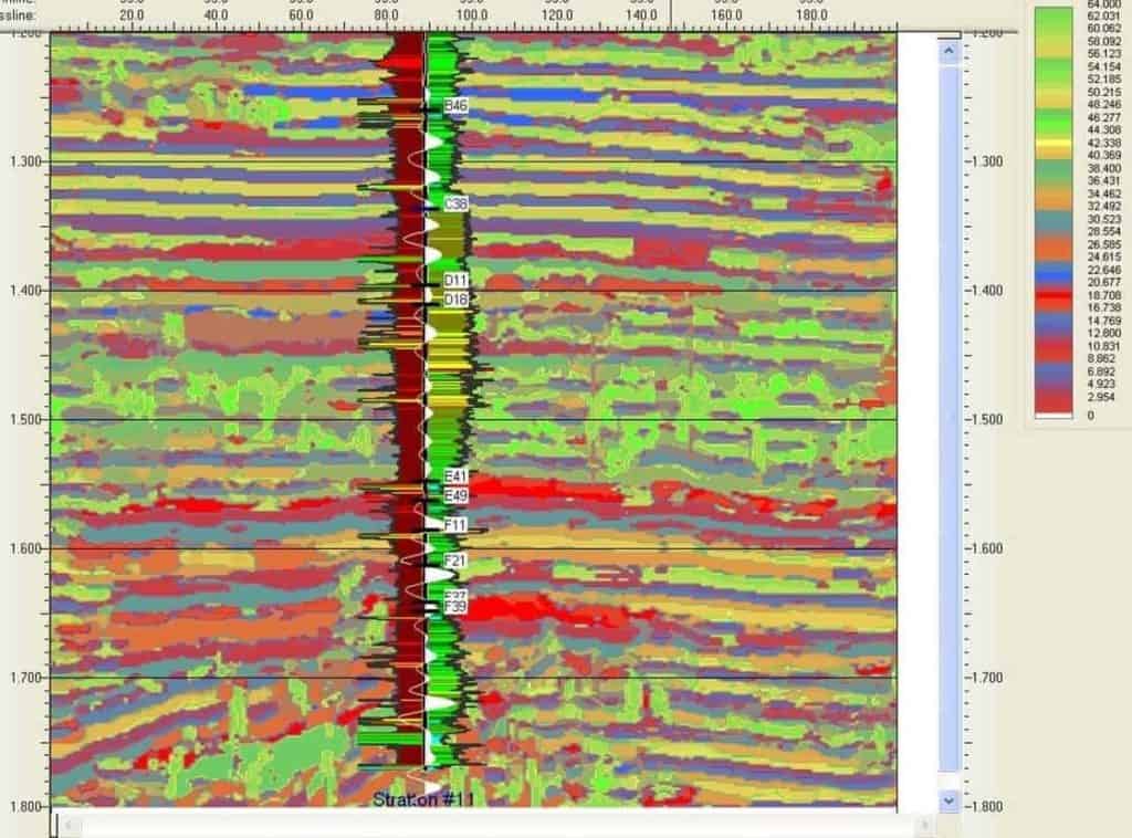
The SOM results form a new attribute volume of winning neuron classifications. Every sample in this new volume is the index of the winning neuron number for a given data sample. The SOM analysis was derived from 50 attributes which included basic trace attributes, geometric attributes and spectral decompositions. A solution line is shown in Figure 5.
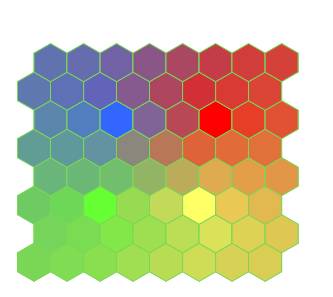
First observe that the SOM results more or less track geology as shown by flat reflections near 1.3s. At the well are shown SP and GR well log curves with lithologic shading, formation top picks as well as a synthetic seismogram (white WTVA trace along the borehole). A second reflector above 1.6s is a second key marker. Also notice the green patches near 1.5s. These were identified as patches with lateral consistency. We have no geologic interpretation at this time. In Figure 6 we show the colorbar patterned to the neuron topology and colored to assist in identification of regions of neuron clusters.
Curvature measure (CM) of the neurons fell in the range .72 to .9 except for one neuron which had a curvature measure of .26. It was found that this winning neuron resulted from only 8 samples while others had 17 to 139.
We have investigated the CM attribute measure and found that there were 3 poor performing attributes (CM < .2); 4 attributes which we consider questionable (CM ≈ .5) and 43 strong attributes (CM > .8).
Automatic anomaly identification
Equation 9 is the basis on which we classify the quality of classification samples. For any winning neuron, we select samples with probability p which exceed threshold pmin
based on the distance between the winning neuron and its samples, shown here as equation 10. Those samples that are near their winning neuron have higher probability.
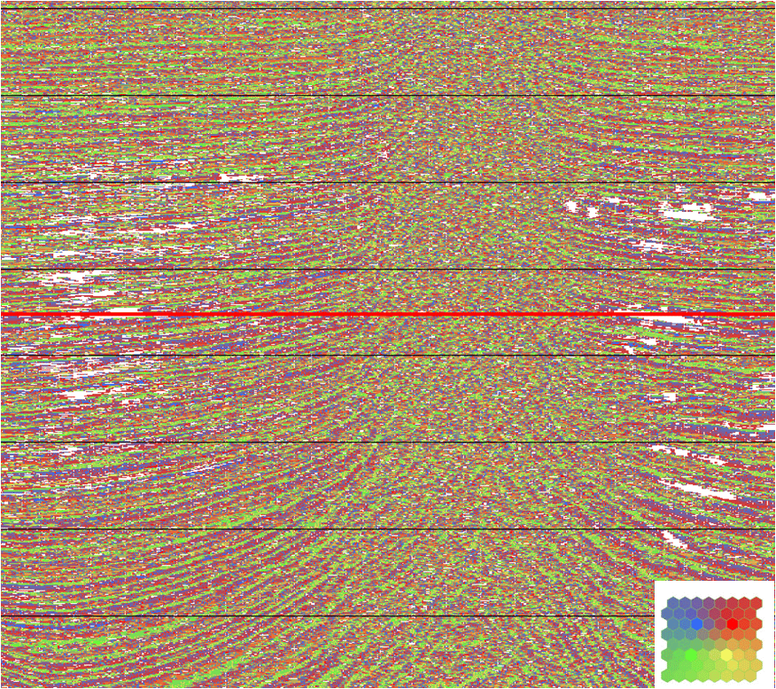
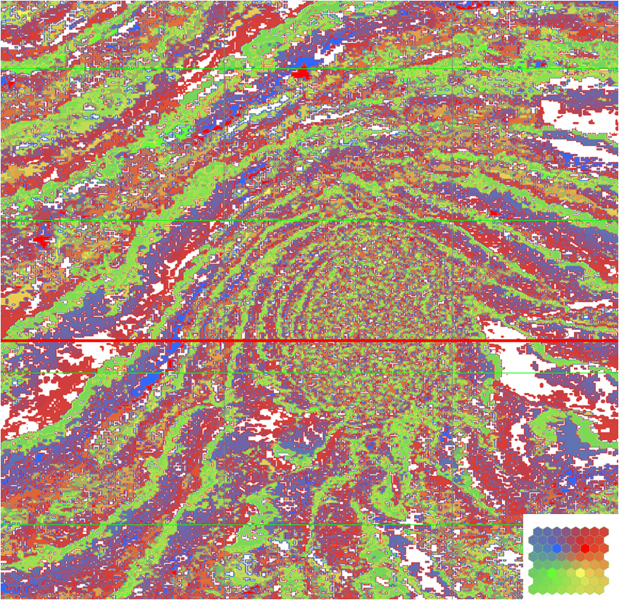
From Figure 7, the classification of Figure 8 results from a SOM analysis with an 8 x 8 neuron network, designed on the basis of F=13 attributes and 100 epochs. Those samples whose probabilities lie below pmin are anomalous and assigned a white color. The rest of the classification uses the colorbar of Figure 6.
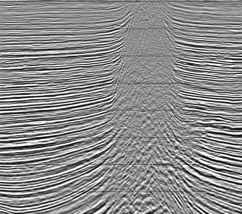
The red lines of Figures 8 and 9 register their views so the white area anomaly on the right side of the salt in Figure 8 has an areal extent that appears to be bounded by the salt in Figure 9. We are not suggesting that all anomalies are of geologic interest. However, those of sufficient size are worthy of investigation for geologic merit.
Conclusion
This presentation investigates the areas within a 3D survey where multiple attributes are of unusual character. Self-organizing maps assist with an automatic identification process. While these results are encouraging, it is readily apparent that additional investigations must be made into appropriate learning controls. Various structural and stratigraphic questions which might be posed to SOM analysis will require careful selection of appropriate attributes. It is also clear that calibration of SOM analyses with borehole information offers an attractive area of investigation.
Acknowledgment
Tury Taner was our inspiration and pioneer in this area.

