Applying Machine Learning Technologies in the Niobrara Formation, DJ Basin, to Quickly Produce an Integrated Structural and Stratigraphic Seismic Classification Volume Calibrated to Wells

Copyright 2022, Unconventional Resources Technology Conference (URTeC) DOI 10.15530/urtec-2022-3701806

This Best of URTeC 2022 paper was prepared for presentation at the Unconventional Resources Technology Conference held in Houston, Texas, USA,
20-22 June 2022.

Abstract

Objectives/Scope: This study will demonstrate an automated machine learning approach for fault detection in a 3D seismic volume. The result combines Deep Learning Convolution Neural Networks (CNN) with a conventional data pre-processing step and an image processing-based post processing approach to produce high quality fault attribute volumes of fault probability, fault dip magnitude and fault dip azimuth. These volumes are then combined with instantaneous attributes in an unsupervised machine learning classification, allowing the isolation of both structural and stratigraphic features into a single 3D volume. The workflow is illustrated on a 3D seismic volume from the Denver Julesburg Basin and a statistical analysis is used to calibrate results to well data.

Methods/Procedures/Process: Starting with a seismic amplitude volume, the method has four steps. Pre-processing produces the volume used as input to the CNN fault classification and the dip volumes used in post processing. Next, CNN applies a 3D synthetic fault engine to predict faults. Then, a directional 3D Laplacian of Gaussian filter enhances the faults in their primary direction and the final step, skeletonization, produces skeletonized probability, dip and azimuth. The result is higher quality when compared to the output from CNN alone (without pre and post processing). The fault volumes are next combined with instantaneous attributes in an unsupervised machine learning classification through Self-Organizing Maps (SOMs) to produce a classification volume from which faults and reservoir neurons can be isolated, calibrated to wells and converted to multi-attribute geobodies.

Results/Observations/Conclusions: The results provide a rapid, robust, and unbiased fault interpretation which can be used to create either fault plane or fault stick interpretations in a standard interpretation package. The SOM is preceded by principal component analysis to identify prominent attributes. These resolve the seismic character of the analysis interval (Top Niobrara to Top Greenhorn). In addition to enhanced fault identification, the Niobrara’s brittle chalk benches are easily distinguished from more ductile shale units and individual benches; A, B, and C benches each have unique sets of characteristics to isolate them in the volume. Extractions from SOM volumes at wells confirm the statistical relationships between SOM neurons and reservoir properties.

Applications/Significance/Novelty: Traditional seismic interpretation, including fault interpretation and stratigraphic horizon picking, is poorly suited to the demands of unconventional drilling with its typically high well densities. Geophysicists devote much of their efforts to well planning and working with the drilling team to land wells. Machine learning applied in seismic interpretation offers significant benefits by automating tedious and somewhat routine tasks such as fault and reservoir interpretation. Automation reduces the fault interpretation time from weeks/days to days/hours. Multi-attribute analysis accelerates the process of high grading reservoir sweet spots with the 3d volume. Statistical measures make the task of calibrating the unsupervised results feasible.

Introduction

As stated in the abstract, applying machine learning technologies to seismic interpretations tasks brings the promise of automation to generating fault volumes through supervised classification. The resulting volumes can subsequently be used to extract fault interpretation.

This methodology is demonstrated in this paper through application to a 100 square mile volume from the Denver-Julesburg Basin. The use of SOMs for isolating chalk reservoirs in the Niobrara was first demonstrated by Laudon and others, 2019. In this study we expand on the original work in two ways: we create a single 3d seismic volume which integrates the result of both machine learning applications, and we calibrate the resulting volumes to well logs via a bivariate statistical analysis following the methodology of Leal and others, 2018.

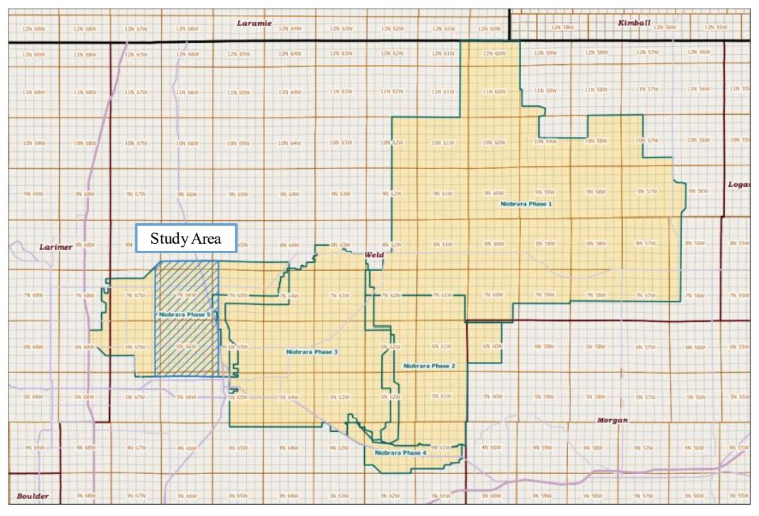
The seismic data are from Phase 5 of a 1580 square mile, contiguous 3D seismic survey conducted from 2011 through 2014 by Geophysical Pursuit, Inc. and Geokinetics (Fairfield Geotechnologies replaced Geokinetics as second data owner). In 2018, the data were provided to Geophysical Insights to conduct proof of concept studies on machine learning techniques for seismic interpretation. Figure 1 shows the location of the study area along with the full outline of the multi-client survey.

Figure 1: Map of Geophysical Pursuit, Inc. and Fairfield Geotechnologies multi-client program and study area outline.

Geologic Setting of the Niobrara and Surrounding Formations

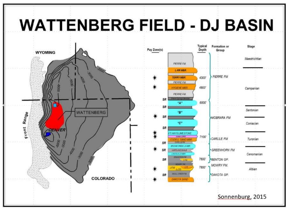
The Niobrara formation is late Cretaceous in age and was deposited in the Western Interior Seaway (Kaufmann, 1977). The Niobrara is subdivided into basal Fort Hays limestone and Smoky Hill members. The Smoky Hill member is further subdivided into three subunits informally termed Niobrara A, B, and C. These units consist of fractured chalk benches which are primary reservoirs with marls and shales between the benches which comprise source rocks and secondary reservoir targets (Figure 2). The Niobrara unconformably overlies the Codell sandstone and is overlain by the Sharon Springs member of the Pierre shale. The Codell is also late Cretaceous in age, and unconformably underlies the Fort Hays member of the Niobrara formation. The interval used for the machine learning studies was Top Niobrara to Top Greenhorn. Figure 2 (Sonnenberg, 2015) shows a generalized stratigraphic column and a structure map for the Niobrara in the DJ Basin along with an outline of the basin, the location of the Wattenberg Field and the approximate location of the study area.

Figure 2: Outline of the DJ Basin with Niobrara structure contours and generalized stratigraphic column that shows the source rock and reservoir intervals for late Cretaceous units in the basin (from Sonnenberg, 2015).

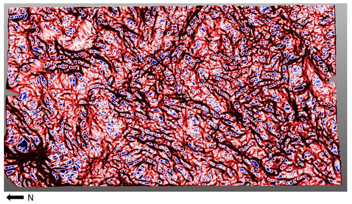
The study area has large antiforms on its western edge as the transition from basin to the Rocky Mountains is crossed. The area is normally faulted with most faults trending northeast to southwest. Landon and others (2001), and Finn and Johnson (2005) have also stated that the DJ basin contains the richest Niobrara source rocks with TOC contents reaching eight weight percent. Niobrara petroleum production is dependent on fractures in the hard, brittle, carbonate-rich zones. These zones are overlain and/or interbedded with soft, ductile marine shales that inhibit migration and seal the hydrocarbons in the fractured zones. Figure 3 shows the most positive curvature, K1 on the top Niobrara. The main fault trends can be seen as well as the potential effect curvature may have on fracturing in the brittle chalk layers.

Figure 3: Most positive curvature, K1 on top Niobrara. There are antiforms present in the lower left (NW) and lower right (SW) portions of the image. The faulting and fractures are complex with both NE-SW and NW-SE trends apparent. Area shown is approximately 100 square miles. Multi-client data shown courtesy of Geophysical Pursuit, Inc. and Fairfield Geotechnologies (from Laudon and others, 2019).

Fault Detection Methodology

Seismic amplitude is the basis for machine learning fault detection which uses deep learning Convolutional Neural Networks (CNNs), a form of supervised machine learning (Ronneberger and others, 2015; Wu and others, 2019; Zhao and Mukhopadhyay, 2018; Qi and others, 2020; Laudon and others, 2021). The results are fault volumes which can be used for seismic fault interpretation. There are different approaches to building a fault prediction engine. This study used CNN engines which were pre-trained using fully 3D synthetic fault models. A 3D synthetic model is unbiased in contrast to manually interpretating faults to build the CNN fault engine (Wu and others, 2019). Models remove the difficulty of picking faults on orientations out of the plane of the faults. Another advantage to using synthetic fault models is that fault prediction is very fast compared to the engine training compute time. The machine learning results are also significantly improved by applying post processing steps of Fault Enhancement and Skeletonization. While Qi and others, 2017, applied this technique to traditional edge detection volumes, we have found that CNN Fault volumes are also ideally suited to this technology. Figure 4 diagrams the high-level workflow consisting of four steps.

Figure 4: Flow diagram for machine learning enhanced fault detection

In step 1, the post stack amplitude data is run through structurally oriented filtering to sharpen discontinuities and further to suppress noise or stratigraphic anomalies sub-parallel to reflector dip. This step significantly improves the fault prediction. This study employed principal component filtering utilizing the University of Oklahoma AASPI consortium algorithms.

Figure 5: Example of Principal Component Structurally Oriented Filtering. Original amplitude, Filtered Amplitude and Rejected Noise. Multi-Client data presented with permission from Geophysicaal Pursuit, Inc. and Fairfield Geotechnologies.

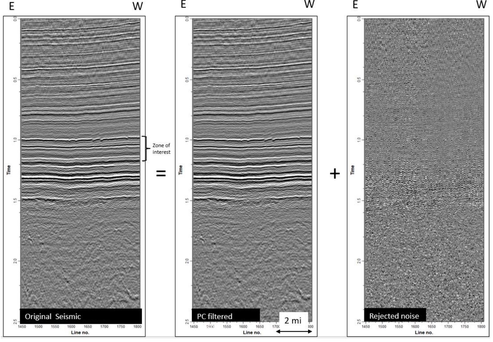
Figure 5 illustrates a faulted amplitude section from the study volume before and after pre-process filtering alongside the rejected noise. The filtering process produces additional volumes, namely Inline Dip, Crossline Dip, and Similarity Total Energy which are required and employed in the post processing steps three and four; fault image enhancement and fault skeletonization and attribute computation (Qi and others, 2017; Qi and others, 2019).

Figure 6 shows the results for steps 2, 3 and 4 of the process. Step 2 is the machine learning fault prediction utilizing fault engines built from 3d synthetic seismic data using convolutional neural networks. Steps 3 and 4, the fault enhancement and skeletonization follows the methodology of Qi and others, 2017 and Qi and others, 2019. This fault image post-processing technique computes and decomposes the second-moment tensor to find the orientation of fault anomalies in the CNN fault probability volume. The 3D directional Laplacian of Gaussian (LoG) filter is then applied to smoothplanar features of the images. The fault anomalies through the direction that is parallel to the faults can be enhanced by the Gaussian operator and sharpened by the Laplacian operator. After that, the faults are skeletonized through the direction that is perpendicular to a given faults. The fault enhancement and skeletonization post-processing step can enhance planar features such as faults and suppress false positives that show non-planar features that cut reflectors. The final output from the workflow are three skeletonized fault volumes: fault probability, fault dip magnitude and fault dip azimuth. The output attributes can be combined to further isolate fault sets based on their geometric properties.

Figure 6: Output from CNN fault prediction, Output from post processing, final fault probability co-rendered with amplitude. Crossline 1399.
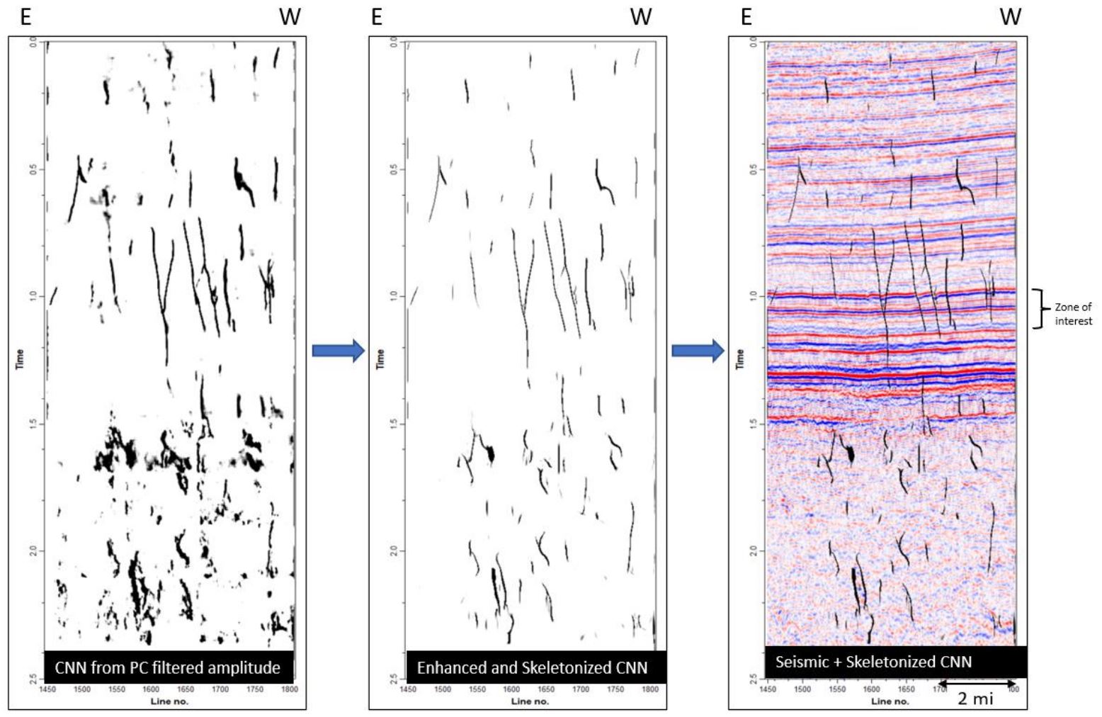
Multi-Client data presented with permission from Geophysical Pursuit, Inc. and Fairfield Geotechnologies.

Unsupervised Classification Utilizing Self-organizing maps (SOM)

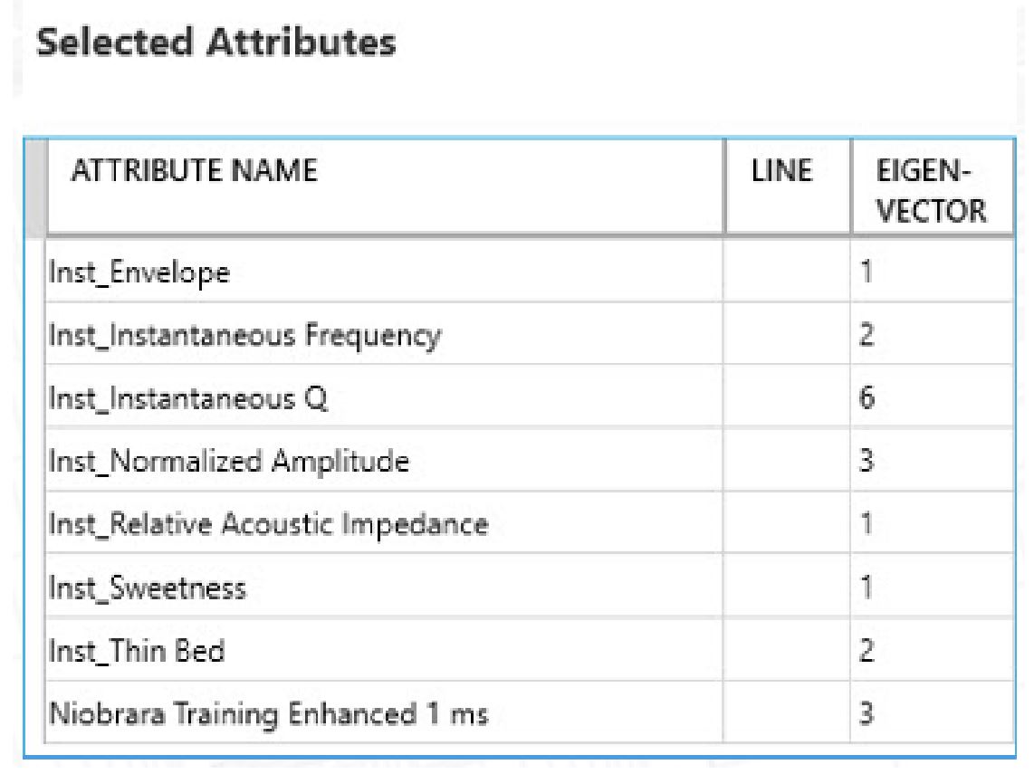
In a previous study, this same seismic volume was used in a stratigraphic machine learning study which yielded detailed stratigraphic information via a multi-attribute classification technique, SOM (Laudon and others, 2019). In that study, nine instantaneous attributes from a suite of nineteen were selected via Principal Component Analysis (PCA). PCA is a linear dimensionality reduction technique frequently used in multi-attribute analysis to determine which attributes are most prominent in the data volume of interest (Roden and others, 2015). SOM is an unsupervised neural network classification which employs a non-linear approach to find natural clusters in multi-dimensional attribute space (Kohonen, 2001; Roden and others, 2015). SOM takes advantage of the organizational structure of the seismic data samples which are highly continuous, greatly redundant, and significantly noisy (Coleou and others, 2003; Roden and others, 2015). The samples from multiple seismic attribute volumes exhibit natural clusters with significant organizational structure in the presence of noise. The SOM classifications of these natural clusters reveal important information about the structure of natural groups that are difficult to perceive any other way. The SOM classifications reveal geologic features which are essential to the subsurface interpretation (Roden and others, 2015). When seismic attributes are organized in attribute space, the SOM algorithm introduces new samples called neurons which seek out natural clusters in attribute space. Through a series of cooperative and competitive training epochs resulting in a fully trained set of winning neurons of classification, each multi-attribute sample is classified to its nearest winning neuron in attribute space. The winning neurons form a 2D mesh that is illuminated in the final volume with a 2D color map for interactive evaluation. One advantage of SOM over other clustering techniques is that within the 2D color map, winning neurons adjacent to each other in the attribute space of the SOM analysis are also adjacent in the final 2D color map (Roden, and others, 2015).

Table 1 shows the attributes used in the SOM and their corresponding eigenvector (Laudon and others, 2019).

Figure 7 shows the original amplitude data on a N-S oriented inline with the zone of interest, Top Niobrara to Top Greenhorn highlighted and an 8×8 SOM for the same interval and line.

Figure 7: North-South inline showing the original amplitude data (upper) and the 8X8 SOM result (lower) from Top Niobrara through Greenhorn horizons (Laudon and others, 2019). Multi-client data shown courtesy of Geophysical Pursuit, Inc. and Fairfield Geotechnologies.

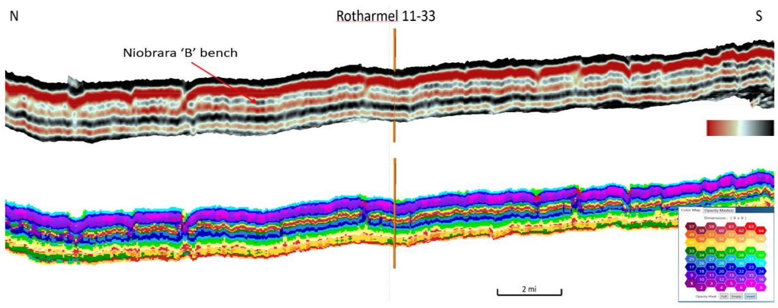
This inline runs through a well with a full suite of logs to correlate and calibrate the SOM results. In this part of the basin, there are three chalks of interest for drilling, A, B, and C, with the B bench having the best reservoir quality. The top Niobrara, on the amplitude section, is a strong peak followed by a broad trough through the highest TOC shale section. The subsequent peak generally corresponds to the B bench. On the SOM classification, the B bench can be seen in the yellow and red neurons and if examined closely, would appear to be mechanically different from the overlying marl. By extracting the red neurons only, the sweet spot within the bench can be visualized easily (Laudon and others 2019). In this study, the SOM classification was repeated with the addition of the skeletonized fault attributes. The resulting volume combines the main structural elements with the same level of stratigraphic detail seen in the previous study. The same inline in Figure 7 is shown in Figure 8 with the new SOM results. Although the actual neuron numbers have changed between SOM runs so the 2D color mapping differs, nevertheless, the stratigraphic picture is the same and detail is enhanced.

There several advantages of using SOM to isolate faults:

• SOM normalizes the input volumes into discrete values allowing easy isolation and interrogation of the seismic volumes to visualize faults.
• Fault volumes from multiple engines (aggressive and conservative) can be combined into a single volume.
• Neuron-derived classifications can be converted into geobodies of common classification. These can be filtered by size if desired and used in a fault extraction workflow.

The SOM neurons which represent faults appear correct on the vertical section, but the real test of the result is the three-dimensional view of the fault neurons.

Figure 8: 8×8 SOM from inline combining instantaneous and fault attributes (top). Original 8×8 SOM utilizing only instantaneous attributes (Laudon and others 2019). Multi-client data shown courtesy of Geophysical Pursuit, Inc. and Fairfield Geotechnologies.

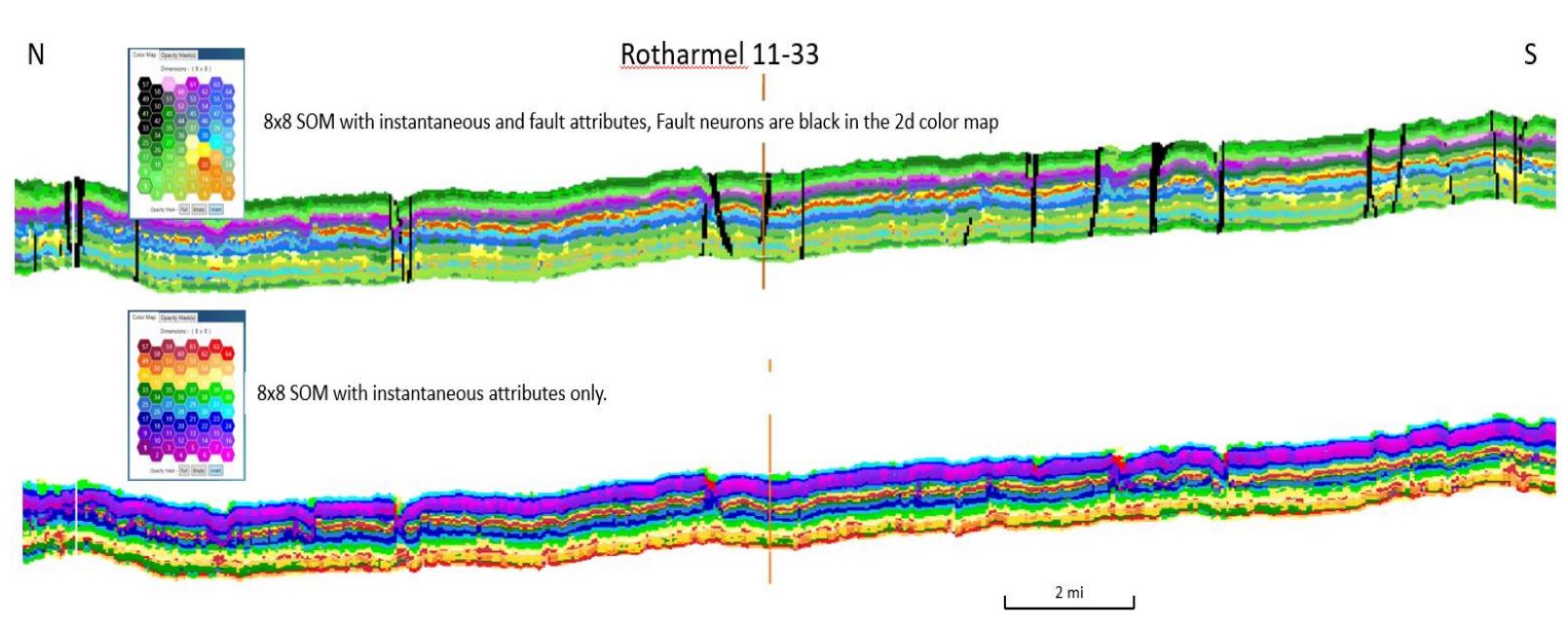
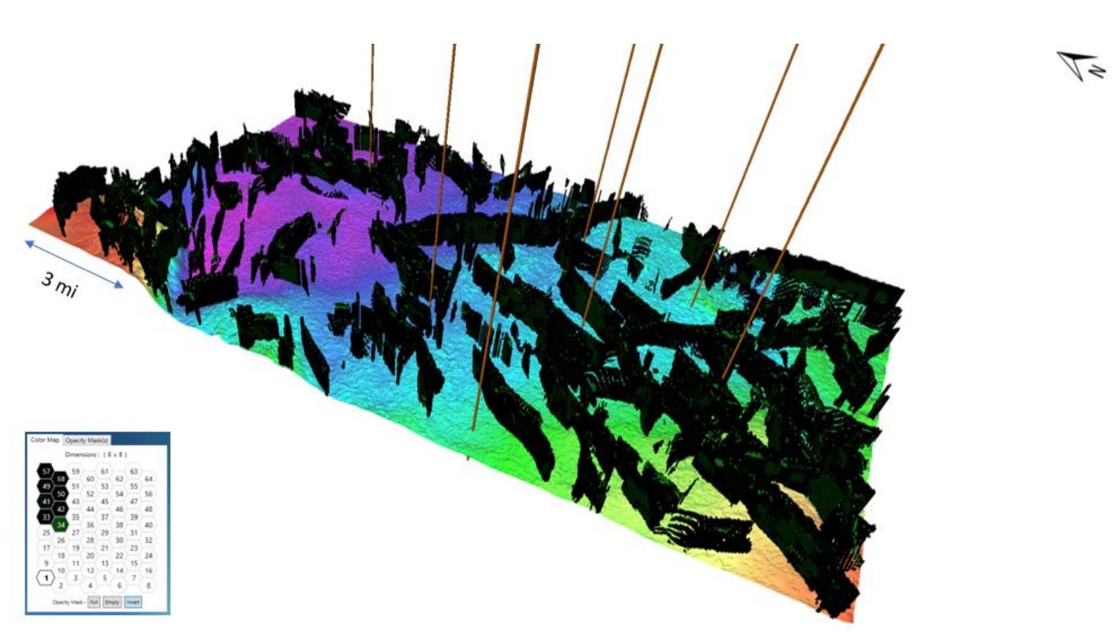
Figure 9 shows a 3D volume of classified seismic samples by a group of SOM fault neurons isolated within the volume using a 2D color map. The position on the color map of the fault neurons demonstrates the self-organizing aspect of natural clustering. The fault neurons are displayed over the Top Greenhorn time structure. The fault results are seen to form well defined fault planes and generally superior to conventional edge detection attributes. The well locations shown are wells which have a full suite of logs and were used for the statistical calibration of the wells to the stratigraphic SOM results as discussed in the next section.

Figure 9: 8×8 SOM result with only neurons representing faults displayed in the 3D volume displayed over the Top Greenhorn time structure. The neurons have been turned black in the 2D color map for contrast and visualization.

Calibration of SOM results to well logs using bivariate statistics

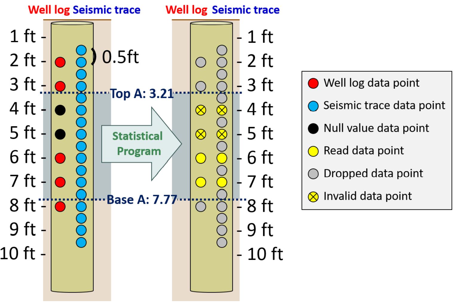
To calibrate the SOM results at well locations, the SOM neuron classifications were extracted at well locations and converted to measured depth using the same sampling interval as the wireline logs (0.5 ft). To combine the SOM neurons extracted from machine learning results and the reservoir properties discriminated from well logs, a contingency table consisting of two categorical variables, SOM neurons and Reservoir, was first created. Two subcategories of Reservoir: Non reservoir and Net reservoir, were determined by applying simple cutoffs to the petrophysical logs (Leal and others, 2018). The well log samples which pass the given petrophysical cutoffs were counted as Net, otherwise they were counted as Non reservoir. Figure 10 shows a schematic of data selection for further statistical analysis. Only data which are valid in both SOM classification and well logs are selected, and others, such as null values and missing points, are excluded from the statistical analysis to prevent mis-estimation.

The standard Chi-square statistical test of independence was first applied to establish the degree of association between two categorical variables. This test compares the observed frequencies to the expected frequencies (the value which was expected if the null hypothesis is true) and determines if there is a statistically significant relationship between variables or not. In this study, the null hypothesis states that two categorical variables are independent (no association between variables), against the alternative hypothesis that they are dependent (the statistical association between variables existed). If the calculated Pearson Chi-square (Chi2) value is higher than the theoretical Pearson Chi-square value (or the calculated p-value is less than the significant level), the null hypothesis is rejected and the alternative hypothesis is accepted. In other words, the occurrences of SOM neurons and the presence of Reservoir are tested for statistical dependence. Another standard statistical measure, natural logarithm of likelihood ratio, applied in this study to test independence is the G-test which measures the difference of the proportions between two categorical variables.

Figure 10: The schematic of data selection for statistical analysis

While these two tests of independence indicate two nominal variables are dependent, the statistical values don’t measure the strength of the relationship between variables. Hence, Cramér’s V, which quantifies the association between two variables by giving a value between 0 and 1, and the Bayes factor, which shows the evidence of a statistical relationship between variables by giving a ratio of the likelihood of the data under each of the two hypotheses, were also calculated. Additionally, to avoid violating the assumptions for the tests as well as the risk of overly optimistic computation of the Chi-square value, the original Nx2 contingency table was converted to a 2×2 contingency table (Table 2) as well as the odds ratio, which quantify the strength of the association between two categorical variables as a ratio of the odds of each category on one variable over the other, was calculated.

Table 2: The schematic of the converted 2×2 contingency table

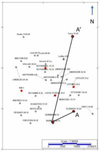
Figure 11 is a map showing the vertical well control in the study area. Seven (7) wells highlighted in red had petrophysical results available for calibration (Holmes and others, 2019). Three wells circled in black in the map are shown in cross section in Figure 12 (A-A’).

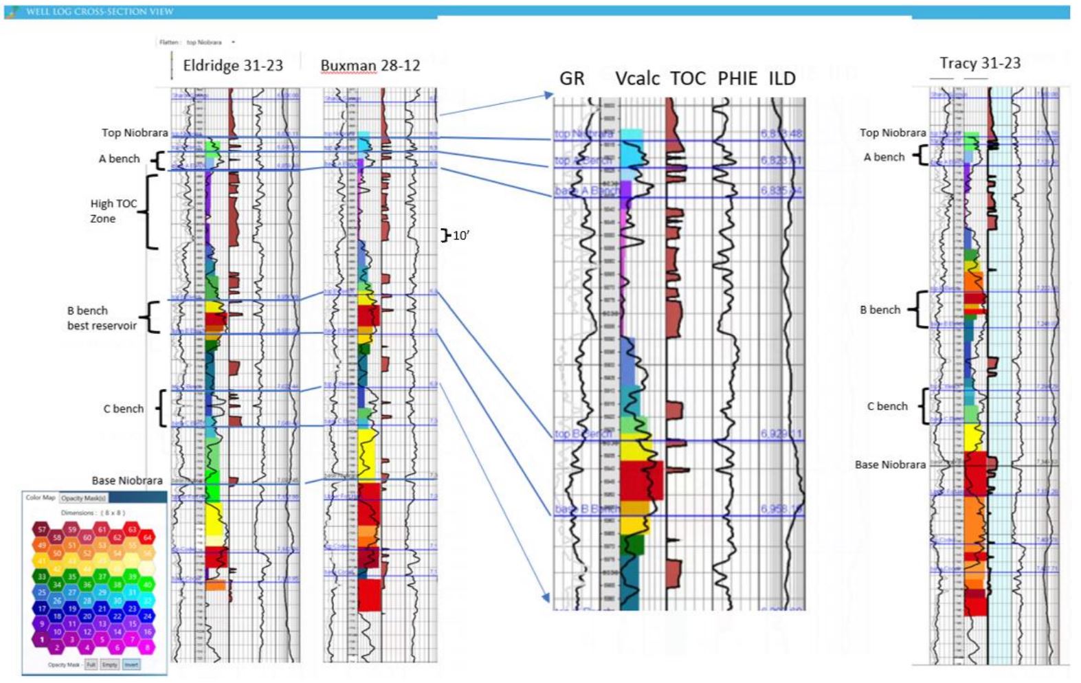
The log template in Figure 12 contains 6 tracks and the cross section is flattened on the Top Niobrara. Track 1 (from left to right) displays Gamma Ray (black) and Vshale (gray); Track 2 is measured depth, Track 3 contains an 8×8 SOM extracted at the well, with the 2D color map used shown in the lower left. The SOM is overlain in Track 3by the Volume of Calcite (Vcalc); Track 4 is Total Organic Content (TOC), Track 5 is Effective Porosity (PHIE) and Track 6 is Deep Induction Resistivity (ILD). The Buxman 28-12 well is expanded to provide a more detailed view of the visual correlation between the individual logs and SOM neurons.

A visual examination shows that the neuron boundaries tie closely to formation tops and transitions in lithology indicator logs, GR, VCalc and TOC. The highest neuron numbers (reds and oranges) indicate high Vcalc and there is a high TOC zone near the Top Niobrara that corresponds to low neuron numbers (pink, purple) in the 2D color map.

Figure 12: Cross section A-A’ showing the Niobrara formation tops, well logs and SOM neurons. Note that the base Niobrara marker only includes the Smoky Hill member and excludes the Ft. Hays limestone.

Using the viusal correlations, the logs selected for the statistical analyses were Vcalc with a cutoff of >0.3 and PHIE with a cutoff of >.03. Net pay was also calculated using a cutoff of Water saturation (Sw) <0.7.

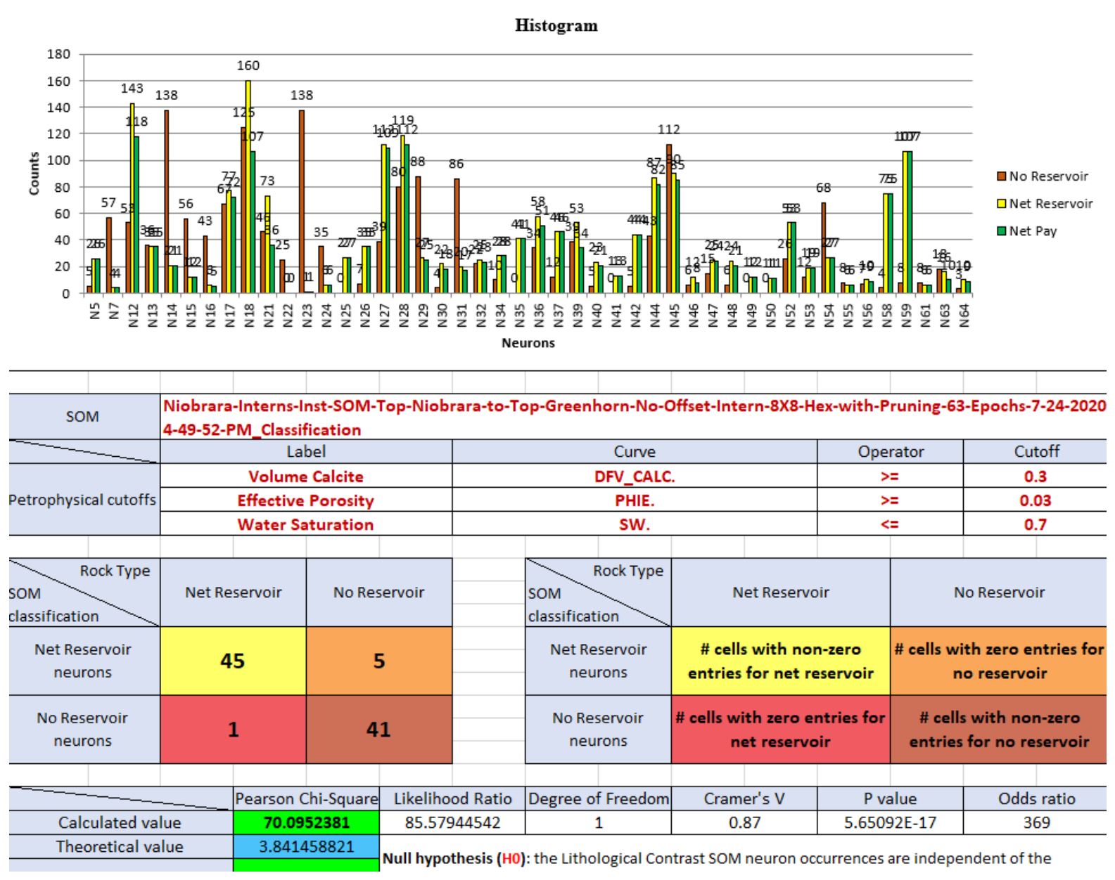
The histogram and Chi2 table in Figure 13 are based on the Smoky Hill portion of the Niobrara section and present each of the 64 neurons in the SOM which were encountered by any of the 7 wells. The histogram parts indicate non-reservoir (brown), net reservoir (yellow) and net pay (green). Hit counts are posted above each histogram bar. The histograms give quick visual indicators of which neurons are the most prevalent (Neuron 18) as well as indicating specific neurons that are strictly non reservoir (Neuron 23) and some which are almost entirely reservoir (Neuron 59).

The Chi2 value for this zone is 1172.9 and the theoretical Chi2 values is 61.6. Therefore, the null hypothesis is rejected, and we safely conclude that there is a strong statistical relationship between SOM neurons and the presence or absence of net reservoir (Leal and others, 2019). The converted 2×2 contingency table summarizes the number of neurons in the well samples which contain reservoir and the number of neurons in the well samples which contain non-reservoir (45 and 41 respectively).

Figures 14-16 show the statistical results for each Niobrara chalk bench individually as well as a 3D view of the neurons associated with each bench, A, B and C. By extracting the SOMs at well locations, we can use the histograms to view the 3D distribution of the neurons assemblages for each bench as determined at well locations. It is worth noting that since seismic samples have higher areal density than wells, there can be samples within a given zone that didn’t necessarily get sampled at all by wells.

Figure 13: Histogram of the Smoky Hill Member of the Niobrara Formation sampled at 7 vertical well locations. The table beneath the histogram lists the SOM neurons used in the calculation, the logs used for petrophysical cutoffs, the confusion matrix, the Chi2 value (calculated and theoretical), likelihood ratio, degrees of freedom, Cramér’s V, P value, and odds ratio. The table also indicates whether the Null hypothesis is accepted or rejected.

Note that the results of Chi2 tests of B and C benches (Figures 15 and 16) indicate that the Null hypothesis is accepted. Statistically here, SOM classifications do not correlate with well classifications. We investigate further to understand what acceptance of the Null hypothesis means. Note from histograms in these figures that there are many net reservoir samples but a lack of non-reservoir samples. While this may provide excellent reservoir results, these results offer poor statistics. A common rule of practice for the Chi2 test of independence is that 80% of cells in large tables in an analysis have 5 or more samples, and further that there are no cells with zero expected counts (see Pearson’s chi-squared test). As we note in these two cases, histograms show that both B and C benches have cells with no samples of non-reservoir classification (in most cases) and several neuron cells have no samples with reservoir. This leads to a failure of the test of independence, and it is due to pushing the statistics too far: these restricted zones of interest had too few samples of certain classifications for reliable statistical conclusions. We note however, that these histograms are still valuable because, along with the 2D colormap and a 3D display, reservoir elements are visualized with winning neurons for each bench.

Figure14: Histogram, Chi2 table and 3D view of neurons in the histogram for the A bench. The Null hypothesis is rejected for this zone. The histogram aids in selecting neurons to isolate in the 3D view.

Figure 15: Histogram, Chi2 table and 3D view of neurons in the histogram for the B bench. The histogram aids in selecting neurons to isolate in the 3D view. Note that the Null hypothesis is accepted in this case, but the visual histogram establishes that the zone is almost 100% reservoir.

Figure 16: Histogram, Chi2 table and 3D view of neurons in the histogram for the C bench. The histogram aids in selecting neurons to isolate in the 3D view. Note that the Null hypothesis is accepted in this case, but the visual histogram establishes that the one is almost 100% reservoir.

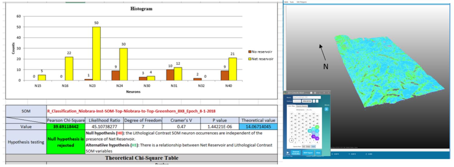
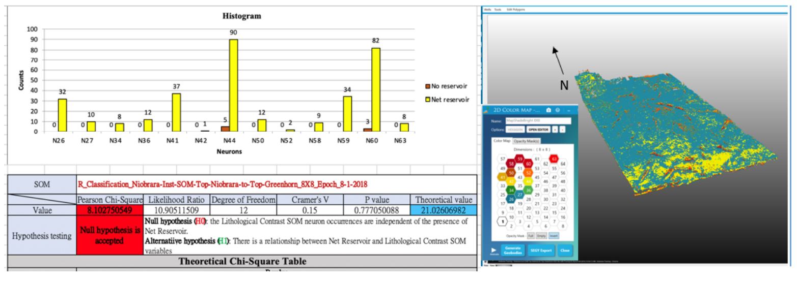
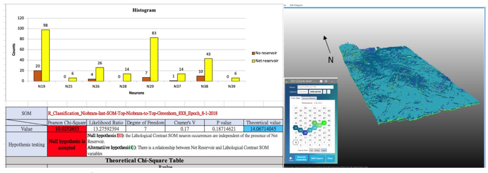
Each chalk bench is represented by a unique assemblage of neurons which is likely a reflection of differences in lithology, porosity and thickness. The neurons representing the A and C benches are closer in the 2D color map and share some of the same neurons meaning that in attribute space, the natural clusters represented by the neurons are nearer each other than those representing the B bench. In general, the B bench is a better reservoir with thicker chalk and slightly higher porosity when compared to A and C. By isolating the individual neurons for each bench, new seismic volumes representing each reservoir can be created and used for volumetrics and well planning.

Conclusions

This paper demonstrates that orchestrated machine learning technologies through a succession of processes has demonstrated the ability to automatically isolate faults and stratigraphy within a single seismic volume and further to link these results to well logs in a statistical, quantitative manner. The machine learning results shown provide a rapid, robust, and unbiased fault interpretation which can be used to create either fault plane or fault stick interpretations in a standard interpretation package. The SOM was preceded by principal component analysis to identify prominent instantaneous attributes. Two types of SOMs were created, one using only instantaneous attributes that highlight stratigraphy and another using instantaneous plus fault detection results that highlight both faults and stratigraphy. Going forward, the recommended approach is to incorporate the fault volumes into SOMs to produce a single classification volume. The SOM results resolve the seismic character of the analysis interval (Top Niobrara to Top Greenhorn). In addition to enhanced fault identification, the Niobrara’s brittle chalk benches are easily distinguished from more ductile shale units and individual benches; A, B, and C each have unique sets of neurons which can be isolated in the classification volume through utilization of a 2D color map. Extractions from SOM volumes at wells confirm the statistical relationships between SOM neurons and reservoir properties.

Acknowledgments

The authors thank Geophysical Insights for use of the Paradise AI workbench to conduct the analysis as well as insightful review and feedback. We thank Geophysical Pursuit, Inc. and Fairfield Geotechnologies for providing the seismic data and the permission to present the data and results.

Digital Formation created the petrophysical logs (Holmes and others, 2019).