Systematic Workflow for Reservoir Characterization in Northwestern Colombia using Multi-attribute Classification

Introduction

Unsupervised machine learning (ML) with Self-Organizing Maps (SOM) was applied to a 3D seismic reflection survey in an area in Northwestern Colombia, South America to better visualize the reservoir of a newly discovered field. This technology encompasses multiple volumes of seismic attributes which are combined into a single volume of multi-attribute seismic samples. With ML, these data are classified with the statistics of sample interval resolution. It is expected that classified seismic samples associated with many SOM winning neurons can be interpreted as single depositional environments with unique rock properties associated with that winning neuron (Roden et al., 2015; Roden and Chen, 2017). Seismic interpretation skills are vital to this process. Other winning neurons, for example, are recognized as assemblages associated with acquisition footprints and others with seismic noise assemblages. In this study, the SOM results were calibrated to wells that have been drilled to date. Geobodies from these winning neurons, which tied to productive intervals registered in these wells, were then visualized for their thicknesses and areal extents within the reservoir field. A workflow is presented which includes data conditioning, finding the best combination of attributes for ML classification aided by Principal Component Analysis, unsupervised ML through SOM multi-attribute seismic sample training and then survey classification in the zone of interest and, finally, geobodies created from classified samples of selected winning neurons, Vizualization of these results are outlined in this paper. The result are potential reservoir estimates calculated through geobodies which have been interpreted with unsupervised ML classifications.

About the study area

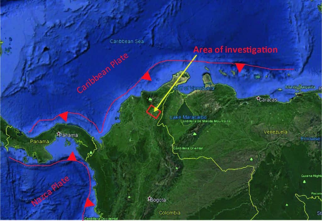
The tectonic setting of this study is along the northwestern margin of South America where the South American plate overrides subduction of the Caribbean Plate. Most specifically, the field discovery occurs within the San Jacinto fold belt, which is a west-verging fold and thrust belt where Upper Cretaceous to Eocene marine basin sediments have been preserved (Mora et al., 2017). See Figure 1 for location of this tectonically complicated study.

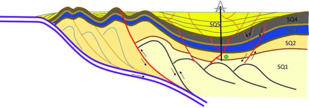
Geologically, the middle to upper Eocene sequence in this area is the Chengue Group. As reported by Mora, et al. (2017), this is identified as Sequence Three out of a total of five identified sequences which comprise the stratigraphy within this fold belt.In the northern portion of the area the Lower Eocene is present, so part of the Chengue formation is in Sequence 2 in the study area.

Figure 2 is a simplified structural rendering of these sequence boundaries. In the figure, SQ2 is the zone of interest in this study. The Sequence Two zone consists of conglomerates, lithic sandstone, siltstones and carbonates.

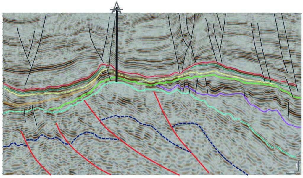
In this tectonically complex area, seismic reflections are complicated as well. Seismically however, the field was found on a paleo-high which, during Eocene time, had a thickness between 100 ft (30.5 m) to 300 ft (91.4 m). Figure 3 shows a typical dip line through the seismic survey to reveal the approximate structural setting of the field. To date, eight wells have been drilled to intercept the Eocene pay zone in the field. Of those eight wells, seven have been found to be economic reservoirs and the eighth well had reservoir rock, but the pay was thin and sitting on water.

Project scope

The goal of this project was to generate a seismic facies model within the zone of interest to improve placement of future wildcat
and development drilling locations within the existing field by implementing unsupervised ML classification techniques. This workflow would allow for evaluation of potential added value of ML-assisted seismic interpretation in areas with complex geologic settings.

Machine learning workflow

Critical to interpretation of sample-based, multiple attribute classification is getting correct time/depth relationships into the wells of interest. For this requirement, individual synthetic seismic relationships between borehole depths and two-way seismic travel times were built for each well borehole. In that way, productive zones at known borehole depths were tied to specific winning neurons in the neural analysis.

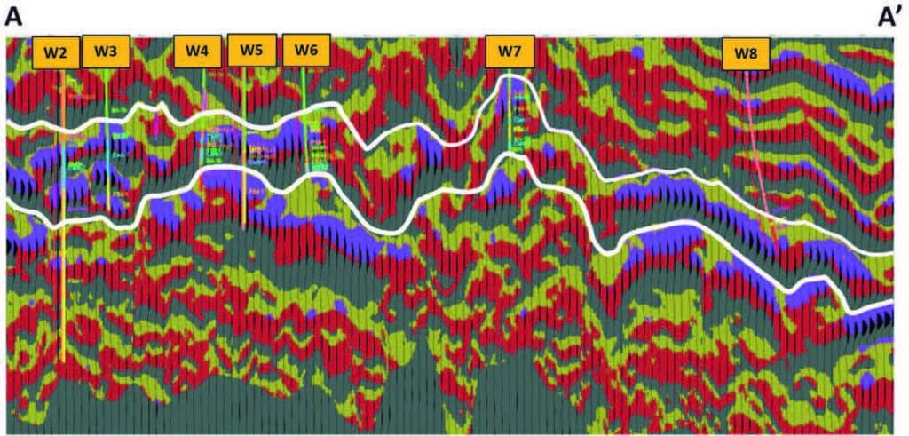
Another important factor for successful seismic interpretation is selection of zones of interest for ML classification which, here, are bounded as pairs of horizons for each zone. Initially the horizons were picked on a 50 m x 50 m inline and crossline grid in the data set across a little over 300 km2. Those grids were then gridded to create a complete surface, and that surface was then converted back to a horizon on all bin locations. Such a loosely-picked smooth grid was then a guide to identify the actual surface around the field area. In a novel approach, the upper surface of the horizon was reinterpreted as guided by a low-topology SOM classification in order to delineate features of sequence boundaries. Figure 4 shows an example of revised upper and lower horizons along an arbitrary line through the well boreholes that were interpreted with the assistance of the low topology SOM training and classification.

Because the field is producing primarily gas with limited liquid hydrocarbons, it was determined that the far angle stack amplitude volume would be used to generate the 17+ attributes used in this analysis. The far angle stack range was from 17 to 26 degrees incident angle at target. In addition to a full suite of instantaneous attributes, very specific geometric attribute volumes were computed to identify faulting and fracturing that might affect the reservoir. The use of the Far Angle Stack volume helped to accentuate any gas response coming from the reservoir. Once the attributes were generated, Principal Component Analysis (PCA) was used to help differentiate those attributes which carried the largest amount of variance and would be the most useful in the classification process to help understand the deposition of the Sequence Three rocks and the hydrocarbon- bearing reservoir within that sequence.

PCA is one of the most common descriptive statistics procedures used to synthesize the information contained in a set of variables. Here PCA of volumes of seismic attributes are reduced in dimensionality through the attribute selection. When applied to seismic attributes, PCA is used to identify those attributes which have made the greatest ‘contribution’ based on the extent of their relative variance to a zone of interest. Attributes identified through PCA are responsive to specific geological features such as lithology changes or fracture zones.

From PCA analysis, five attributes were selected for the SOM analysis. Those were Normalized Amplitude, Instantaneous Phase, Envelope, Hilbert and Sweetness, all of which were calculated from the far angle stack, as mentioned previously. Each of these attributes within the defined window of investigation was then ‘normalized’ to one another so that no one attribute carried more weight of information than any other attribute. Then during SOM training, that sample information which was organized into distinct natural clusters (patterns) by the vectors (neurons) in an attribute space is identified and classified. After training, all multi-attribute seismic samples are classified by these trained winning neurons and displayed by a 3D viewer. Each classification pattern is isolated and viewed in a 3D volume visualizer using the 2D colour map. The colour map is based on the SOM neural network which has adapted to the multi-attribute training samples.

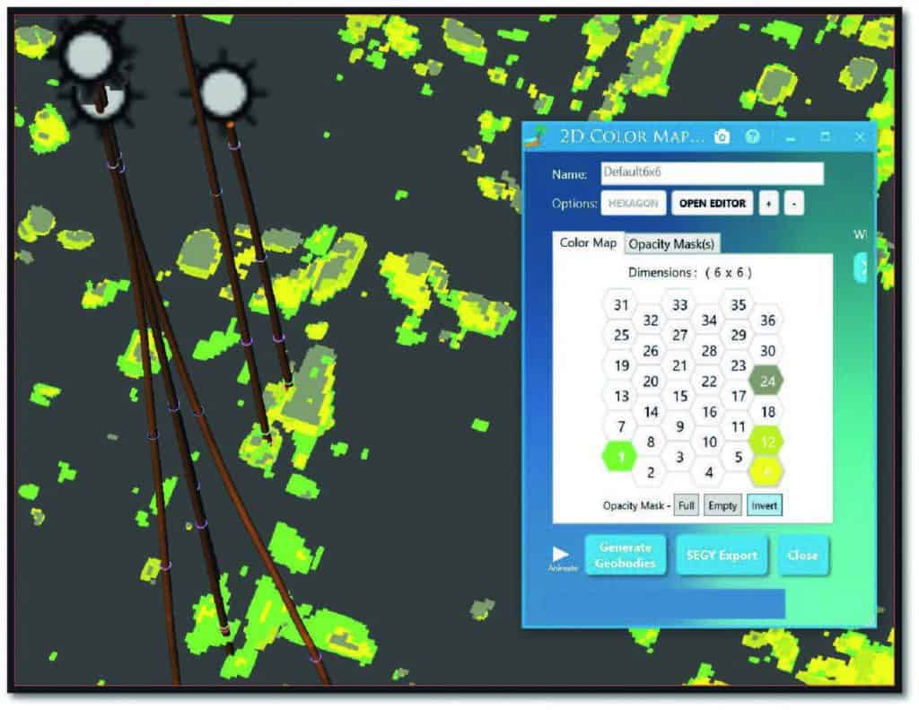
Figure 5 illustrates the value of individual classification patterns within a volume. One reason for unsupervised SOM is that there is no way of knowing the number of natural ‘patterns’ that occur within the investigation window.Instead of forcing a solution to a model of a fixed number of classifications, the data itself defines the information picked by ML from natural clusters of samples of similar seismic attributes as they occur in the actual data. Often, several SOM neural network topologies, showing different levels of detail, are used in the seismic interpretation of geologic features to better determine lithology details. This work included multiple neural network topologies to arrive at an optimum. Using too few winning neurons combines natural clusters, resulting in only a gross picture of the reservoir, while too many winning neurons will produce an image of the subsurface with so much detail it is difficult to interpret.

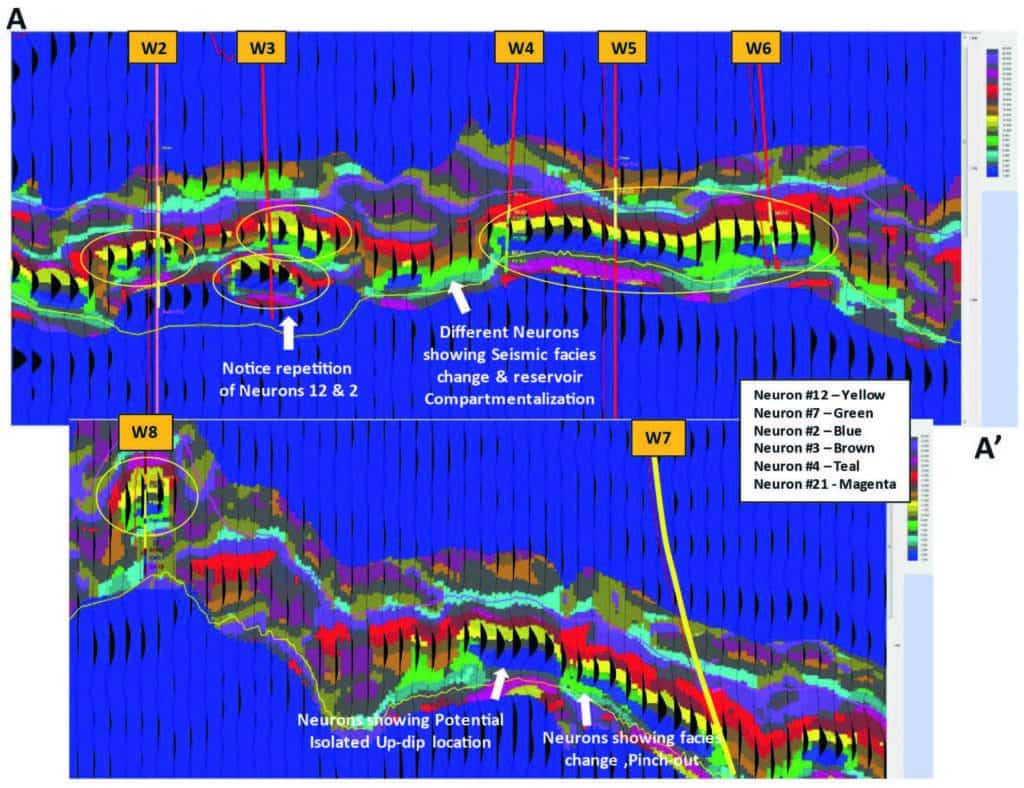
A series of neuron topologies were generated and evaluated ranging from 2×2 (for mapping purposes only) through to 9×9. The chosen topology best tied SOM classifications to well control lithologies extracted from the log lithofacies – a 5×5 neuronal topology with 25 winning neurons. Figure 6a shows an enlarged portion of an arbitrary line through five wells in the field. The key winning neurons are listed with their comparative colours in the 2D Colormap colours. In Figure 6a three wells appear to be in the same reservoir (wells W4, W5, and W6), while two wells (W2 and W3) are compartmentalized in another portion, although both are in the same lithologies as inferred from their classification. Figure 6b (bottom) shows the remaining portion of the arbitrary line that passes through well W8 which was identified as a slightly different reservoir component by SOM classification with dark-yellow Neuron #11. Well W7 was the single well which was drilled downdip to the main portion of the field and interpreted here as only clipping a portion of the reservoir, which at that point was on water (personal communication – Sierra).

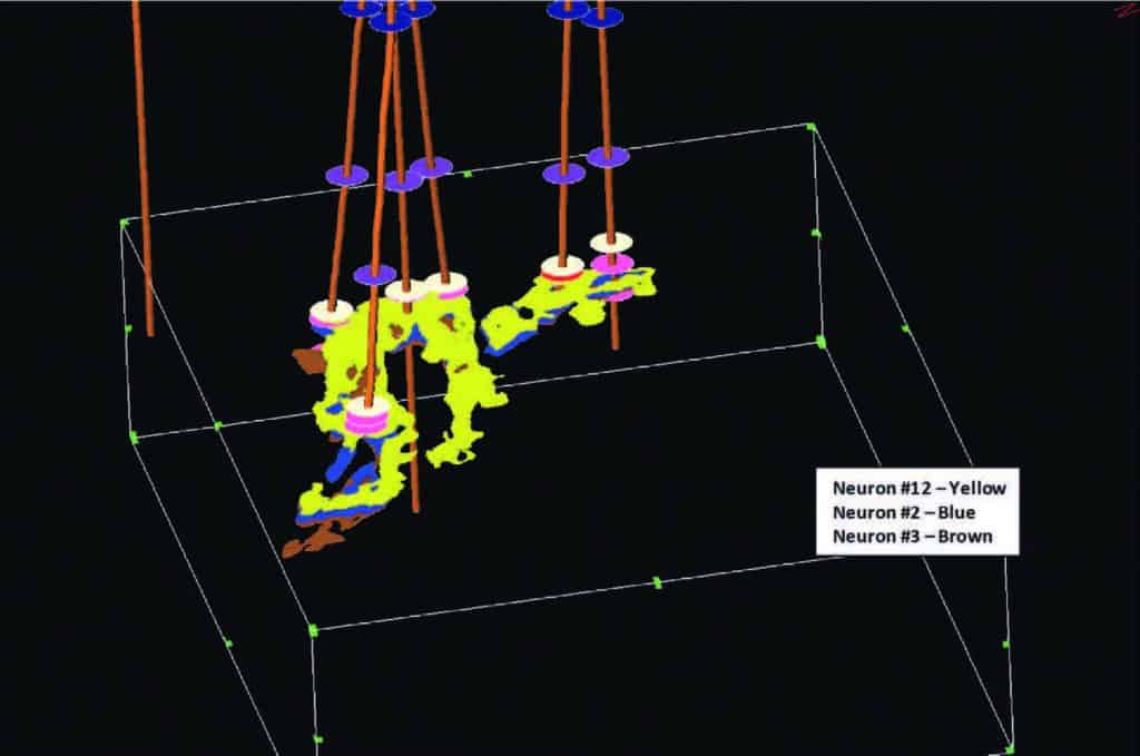
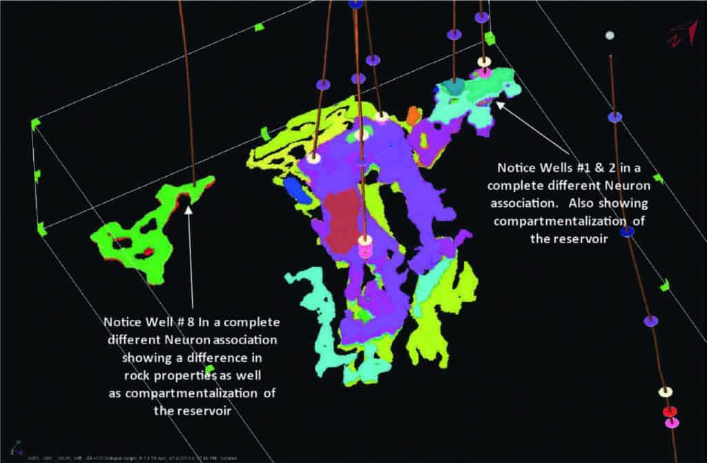
Once it was determined that the 5×5 neuron topology SOM calibrated best to well control, geobodies were identified in the classified seismic samples associated with selected winning neurons listed in Figure 5. The main reservoir classified samples associated with winning neurons, #2, #3 and #12 are seen in the 3D visualization display in Figure 7, while all classified samples associated with the winning neurons linked to production can be seen in Figure 8.

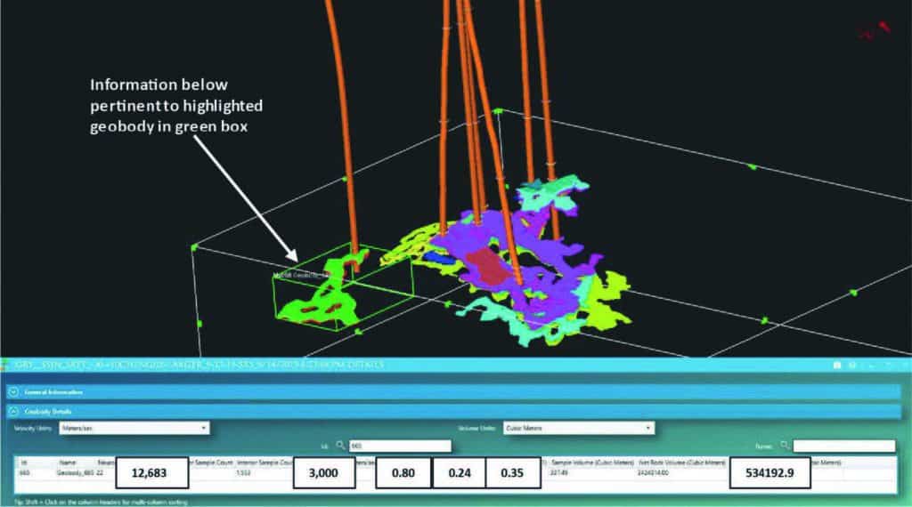
Once selected geobodies have been identified with specific portions of the reservoir, a table is easily constructed so that potential reserves can be calculated within the interpreted geobody. These potential reservoir calculations require several pieces of information, namely interval velocities, net to gross ratios, porosities (in decimal percentages) and water saturation (also in decimal percentage). An example of these calculations is shown in Figure 9. A similar use of SOM sample calculations for reservoir estimation is reported by Leal et al., 2019.

Conclusions

It was determined through this study that the deposition of these reservoirs was discontinuous and compartmentalized. This discovery is contrary to the published interpretation of this unit as ‘Fan deltas and related submarine slope deposits’ (Mora et al., 2017). We interpret this unit as more composed of debris flows or mass transport systems than a fan. This new depositional model matches core data and inferred seismic sample classifications near the wells.

There is evidence from unsupervised ML classifications, that not only lithological information was revealed, but also fluid effect because it was based on the Far Angle survey attributes which could be known to exhibit fluid effect. This was observed near well #8. It was also shown through the classification process that key reservoirs in this area are not limited by structure but have a stratigraphic component as well.

It was advantageous to use unsupervised ML classification of multi-attribute seismic samples because the technology is highly effective at revealing stratigraphic patterns in a complex structural setting. This was not evident from regular seismic amplitude data nor possible to be discovered through a tedious analysis of individual seismic attributes. Winning neuron ML classification has been found in this work and elsewhere to be a cost-effective alternative to traditional seismic inversion projects. The method is both a faster interpretation process with finer details and less subject to rock mechanics sampling limitations. Cost savings aside, the ML classification process also provided a significant time saving in arriving at a seismic interpretation. Zones of interest could be delineated within a matter of a few days instead of the weeks or months typically required for inversion processing of these data. In areas without well control, unsupervised ML classification is an attractive interpretation tool where seismic inversion is not possible because of a lack of subsurface well borehole sampling. This allows interpreters who are assisted by ML classification analysis to improve predictions of depositional patterns, thus helping to reduce risk in provinces of wildcat exploration.

Finally, it must be noted that data preparation before ML is crucial, and can easily take up 70 to 80% of total project time. Particularly important is the time needed to properly determine precise time/depth relationships at the wells to accurately tie borehole lithologies to respective seismic classifications based on ML training of seismic samples near the wells. Moreover, an accurate time/depth relationship is critical for many other successful types of analysis. Unsupervised ML classification based on low neuron topology analysis can aid in mapping difficult depositional and structural environments, and multiple combinations of attributes can help to determine which analysis best fits the wells. This, in turn, results in geobodies of greater dependability whose volumetric calculations may have greater accuracy that can be tested by dynamic reservoir simulation.

Acknowledgments

The authors would like to thank the Lewis Energy Group, particularly Stan Jumper, V.P. Exploration, for allowing the presentation of this study. We would also like to thank Geophysical Research, LLC (d/b/a Geophysical Insights), developers of the Paradise AI workbench, and the team members which facilitated the study including Hal Green, Rocky Roden, Sarah Stanley, Ivan Marroquin, Deborah Sacrey, Camilo Sierra and Diego Sanchez.