Solving Exploration Problems with Machine Learning

Introduction

Over the past eight years the evolution of machine learning in the form of unsupervised neural networks has been applied to improve and gain more insights in the seismic interpretation process (Smith and Taner, 2010; Roden et al., 2015; Santogrossi, 2016: Roden and Chen, 2017; Roden et al., 2017). Today’s interpretation environment involves an enormous amount of seismic data, including regional 3D surveys with numerous processing versions and dozens if not hundreds of seismic attributes. This ‘Big Data’ issue poses problems for geoscientists attempting to make accurate and efficient interpretations. Multi-attribute machine learning approaches such as self-organizing maps (SOMs), an unsupervised learning approach, not only incorporates numerous seismic attributes, but often reveals details in the data not previously identified. The reason for this improved interpretation process is that SOM analyses data at each data sample (sample interval X bin) for the multiple seismic attributes that are simultaneously analysed for natural patterns or clusters. The scale of the patterns identified by this machine learning process is on a sample basis, unlike conventional amplitude data where resolution is limited by the associated wavelet (Roden et al., 2017).

Figure 1 illustrates how all the sample points from the multiple attributes are placed in attribute space where they are standardized or normalized to the same scale. In this case, ten attributes are employed. Neurons which are points that identify the patterns or clusters, are randomly located in attribute space where the SOM process proceeds to identify patterns in this multi-attribute space. When completed, the results are nonlinearly mapped to a 2D colormap where hexagons representing each neuron identify associated natural patterns in the data in 3D space. This 3D visualization is how the geoscientist interprets geological features of interest.

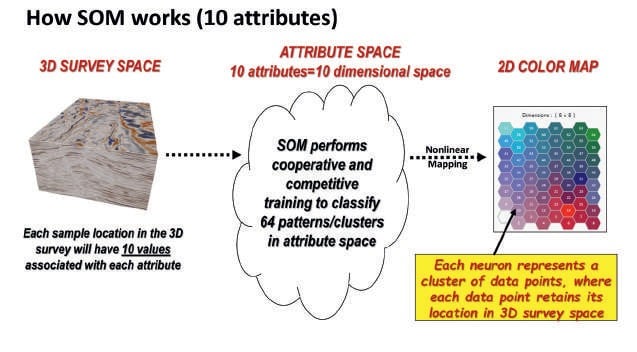
The three case studies in this paper are real-world examples of using this machine learning approach to make better interpretations.

Case History 1 – Defining Reservoir in Deep, Pressured Sands with Poor Data Quality

The Tuscaloosa reservoir in Southern Louisiana, USA, is a low-resistivity sand at a depth of approximately 5180 to 6100 m (17,000 to 20,000 ft). It is primarily a gas reservoir, but does have a component of liquids to it as well. The average liquid ratio is 50 barrels to 1MMcfg. The problem is being able to identify a reservoir around a well which has been producing from the early 1980s, but has never been offset because of poor well control and poor seismic data quality at that depth. The well in question has produced more than 50 BCF of gas and approximately 1.2 MMBO, and is still producing at a very steady rate. The operator wanted to know if the classification process could wade through the poor data quality and see the reservoir from which the well had been producing to calculate the depleted area and look for additional drilling locations.

The initial data quality of the seismic data, which was shot long after the well started producing is shown in Figure 2. Instantaneous and hydrocarbon-indicating attributes were created to be used in a multi-attribute classification analysis to help define the laminated-sand reservoir. The 3D seismic data areal coverage was approximately 72.5 km2. and there were 12 wells in the area for calibration, not including the key well in question. The attributes were calculated over the entire survey, from 1.0 to 4.0 seconds, which covers the zone of interest as well as some possible shallow pay zones. Many of the wells had been drilled after the 3D data was shot, and ranged from dry holes to wells which have produced more than 35BCFE since the early 2000s.

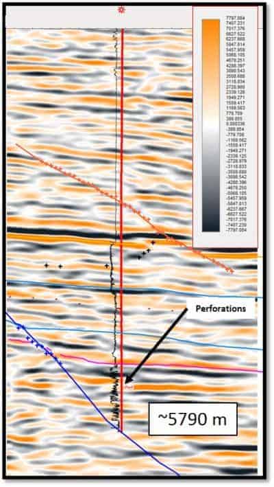
A synthetic was created to tie the well in question to the seismic data. It was noted that the data was out-of-phase after tying to the Austin Chalk. The workflow was to rotate the data to zero-phase with U.S. polarity convention, up-sample the data from 4 ms to 2 ms, which allows for better statistical analysis of the attributes for classification purposes, and create the attributes from the parent PSTM volume. While reviewing the attributes, the appearance of a flat event seemed to be evident in the Attenuation data.

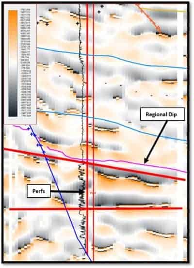
Figure 3 shows what looks like a ‘flat spot’ against regional dip. The appearance of this flat event suggests that a combination of appropriate seismic attributes used in the classification process designed to delineate sands from shales, hydrocarbon indicators and general stratigraphy, may be able to define this reservoir. The eight attributes used were: Attenuation, Envelope Bands on Envelope Breaks, Envelope Bands on Phase Breaks, Envelope 2nd Derivative, Envelope Slope, Instantaneous Frequency, PSTM-Enh_180 rot, and Trace Envelope. A 10×10 matrix topology (100 neurons) was used in the SOM analysis to look for patterns in the data that would break out the reservoir in a 200 ms thick portion of the volume, a zone in which the Tuscaloosa sands occur in this area.

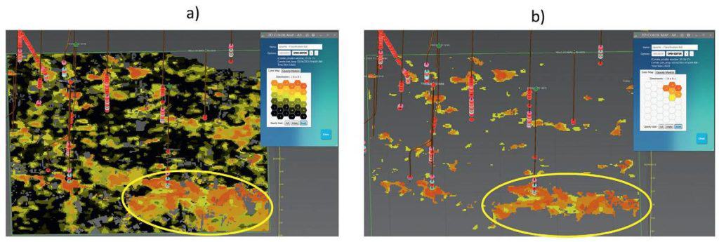
Figure 4a shows a time slice from the SOM results through the perforations with all the neural patterns turned on in 3D space as well as the well bores within the area of the 3D space. Figure 4b shows only the sand reservoir without all the background information. It can be noted that this time slice cuts regional dip in a thinly-laminated reservoir, so evidence of a braided stream system can readily be seen in the slice. Figure 4b shows the same time slice, but with only the key neural patterns turned on in the 2D Map matrix of neurons.

The result is that the reservoir for the key well ended up calculating out to 526 Hectares, which explains the long life and great production. It also seems to extend off the edge of the 3D space, which could add significantly to the reservoir extent.

Case History 2 – Finding Hydrocarbons in Thinbed Environments Well Below Seismic Tuning

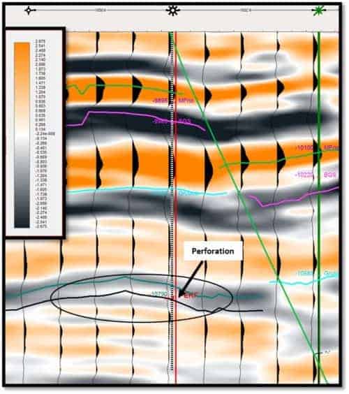
In this case, the goal was to find an extension of a reservoir tied to a well which had produced more than 450 MBO from a thin Frio (Tertiary Age) sand at 3289 m. The sand thickness was just a little over 2 m, well below seismic tuning (20 m) at that depth. Careful attention to synthetic creation showed that the well tied to a weak peak event. Figure 5 shows this weak amplitude and the tie to the key well. Again, the data was up-sampled from a 4 ms sample rate to a 2 ms sample rate for better statistics in the SOM classification process, then the attributes were calculated from the up-sampled PSTM-enhanced volume.

The reservoir was situated within a fault block, bounded to the southeast by a 125 m throw fault and along the northwest side by a 50 m throw fault. There were three wells in the southwest portion of the fault block which had poor production and were deemed to be mechanical failures. The key producer was about 4.5 km northeast of the three wells along strike within the fault block. Figure 6 shows an amplitude strike line that connects the marginal wells to the key well. The green horizon was mapped in the trough event that was consistent over the area. The black horizon is 17 ms below the green horizon and is located in the actual zone of perforations in the key producing well and is associated with a weak peak event.

A neural topology of 64 neurons (8×8) was used, along with the following eight attributes to help determine the thickness and areal extent: Envelope, Imaginary Part, Instantaneous Frequency, PSTM-Enh, Relative Acoustic Impedance, Thin Bed Indicator, Sweetness and Hilbert. Close examination of the SOM results (Figure 7) indicated the level associated with the weak peak event resembled some offshore bar development. Fairly flat reflectors below the event and indications of ‘drape’ over the event led to the conclusion that this sand was not a blanket sand, as the client perceived, but had finite limitations. Figure 7 shows the flattened time slice in the perforated zone through the event after the neural analysis. One can see the possibility of a tidal channel cut, which could compartmentalize the existing production. Also noted is the fact that the three wells which had been labelled as mechanical failures, were actually on very small areas of sand which indicate limited reservoir extent.

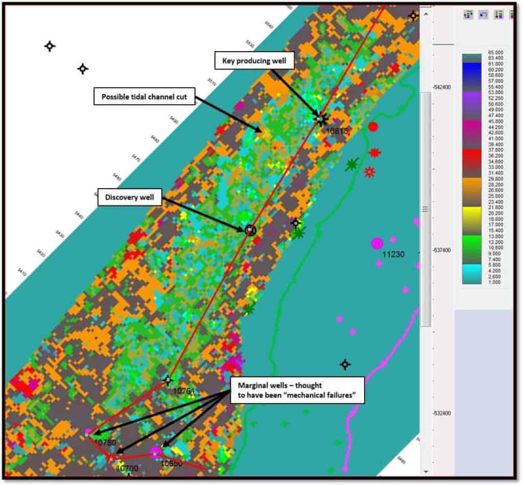
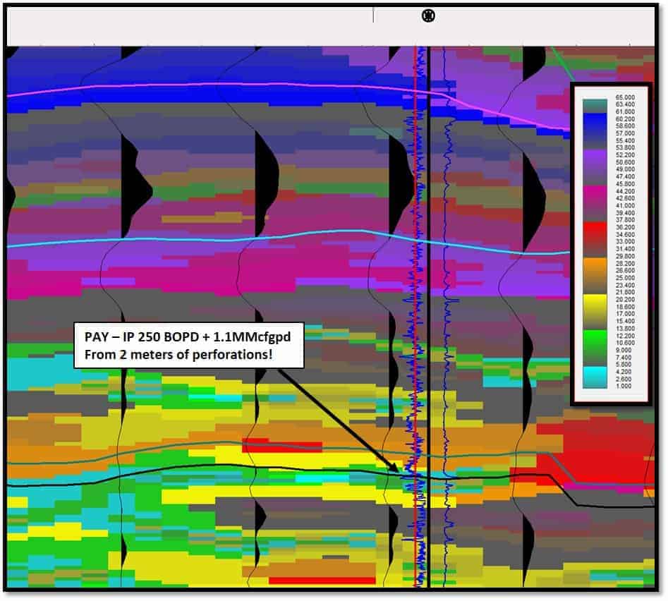
Figure 8 is a SOM dip seismic section showing the discovery well after completion. Three m of sand was in the well bore and 2 m were perforated for an initial rate of 250 BOPD and 1.1 MMcfgpd. The SOM results identified these thin sands with light-blue-to-green neurons, with each neuron representing about 2-3 m thickness. This process has identified the thin beds well below the conventional tuning thickness of 20 m. It is estimated that there is another 2 MMBOE remaining in this reservoir.

Case History 3 – Using the Classification Process to Help With Interpreting Difficult Depositional Environments

There are many places around the world where the seismic data is hard to interpret because of multiple episodes of exposure, erosion, transgressive and regressive sequences and multi-period faulting. This case is in a portion of the Permian Basin of West Texas and Southeastern New Mexico. This is an area which has been structurally deformed from episodes of expansion and contraction as well as being exposed and buried over millions of years in the Mississippian through to the Silurian ages. There are multiple unconformable surfaces as well as turbidite and debris flows, carbonates and clastic deposition, so it is a challenge to interpret.

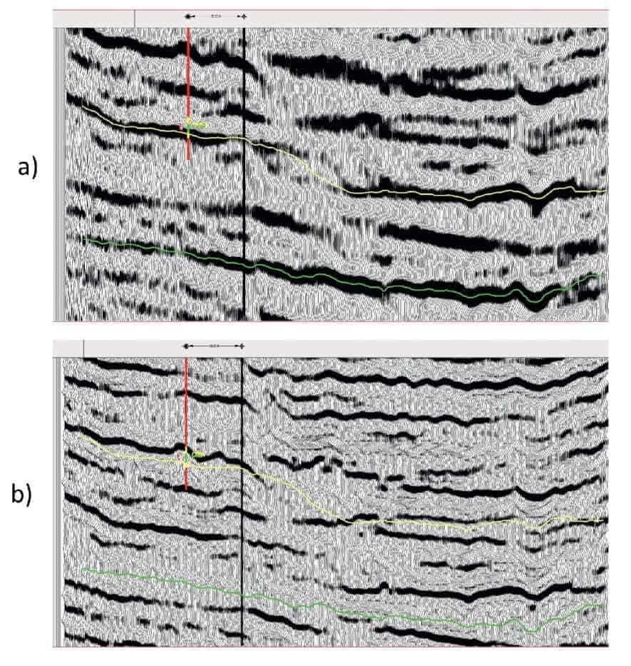
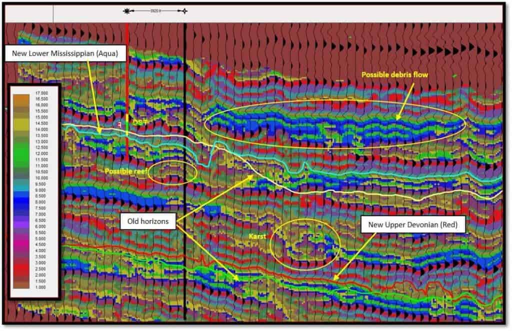
The 3D has both a PSTM stack from gathers and a high-resolution version of the PSTM. The workflow was to use the high-resolution volume and use a low-topology SOM classification of attributes which would help accentuate the stratigraphy. Figure 9a is an example of the PSTM from an initial volume produced from gathers and Figure 9b is the same line in the high-resolution version. The two horizons shown are Lower Mississippian in yellow and the Upper Devonian in green, both horizons were interpreted in the PSTM stack from gathers. One can see in the high-resolution volume that both horizons are definitely not following the same events and additional detail in the data is desired.

The workflow here was to use multi-attribute classification with a low-topology (fewer neurons, so fewer patterns to interpret) unsupervised Self-Organized Map (SOM). The lower neural count will tend to combine the natural patterns in the data into a more ‘regional’ view and make it easier to interpret. A 4×4 neural matrix was used, so the result only had 16 patterns to interpret. The four attributes used were also picked for their ability to sort out stratigraphic events. These were: Instantaneous Phase, Instantaneous Frequency, and Normalized Amplitude.

Figure 10 is the result of the interpretation process in the SOM classification volume. Both the new interpreted horizons and the old horizons are shown to illustrate how much more accurate the classification process is at defining stratigraphic events. In this section, one can see karsting, debris flows and possibly some reefs.

Conclusion

In this article, three different scenarios were given where the use of multi-attribute neural analysis of data can aid in solving some of the many issues geoscientists face when trying to interpret their data. The problems solved were using SOM classification to help define 1) reservoirs in deep, pressured, poor data quality areas, 2) thin-bedded reservoirs while exploring or developing fields and 3) classification of data to help interpret data in difficult stratigraphic environments. The classification process, or machine learning, is the next wave of new technology designed to analyze seismic data in ways that the human eye cannot.

Acknowledgments

The authors would like to thank Geophysical Insights for the research and development of the Paradise® AI workbench and the machine learning applications used in this paper.

References

Roden, R. and Chen, C., 2017, Interpretation of DHI Characteristics with machine learning. First Break, 35, 55-63.
Roden, R., Smith, T. and Sacrey, D., 2015, Geologic pattern recognition from seismic attributes: Principal component analysis and self-organizing maps. Interpretation, 3, SAE59-SAE83.
Roden, R., Smith, T., Santogrossi, P., Sacrey, D. and Jones, G., 2017, Seismic interpretation below tuning with multi-attribute analysis. The Leading Edge, 36, 330-339.
Santogrossi, P., 2017, Technology reveals Eagle Ford insights. American Oil & Gas Reporter, January.
Smith, T. and Taner, M.T., 2010, Natural clusters in multi-attribute seismics found with self-organizing maps. Extended Abstracts, Robinson-Treitel Spring Symposium by GSH/SEG, March 10-11, 2010, Houston, Tx.