Unsupervised vs. Supervised classifiers – Comparing classification results

In machine learning, there is a very interesting challenge in comparing the quality of the classification result generated by either unsupervised or supervised classifiers. Most of the time, we opt for one technique over the other. Sometimes, we perform a comparison study and use a visual examination to decide which classifier produced the best outcome.

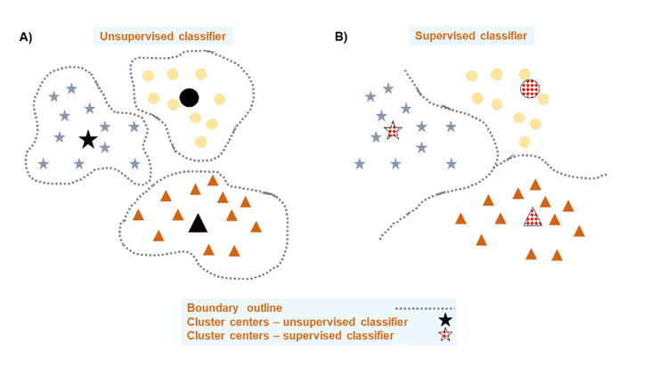
Can we do better than this? I believe so! Let’s assume that we have a dataset that consists of three well-defined groups of data points. Then, we use an unsupervised classifier to generate three clusters. The algorithm produces two outputs: (1) cluster centers and (2) membership of each data point to its closest cluster center. As a consequence, we get the boundaries of clusters (see figure A below). If we present the same data to a supervised classifier, assuming that the data points already have a class label assigned to them, the algorithm generates boundaries that separate a class from each other (see figure B below). So far, you would think: I cannot still compare the classification outputs. However, there is a common trait between these results: the presence of boundaries. What if I tell you that we can take advantage of the notion of the boundaries in the context of supervised classifiers. In a way, it can help to derive cluster centers associated with each predicted class (see cluster center symbols with dashed patterns in red in figure B below).

There are so many different types of classification problems, I focused on the case of lithofacies classification from wireline well log data. I used this data to implement a machine learning pipeline to derive cluster centers. The pipeline consists of three steps (see diagram below): (1) generate a lithofacies classification, (2) derive cluster centers from lithofacies classification result, and (3) validate cluster centers. Each of these steps was addressed with a specific machine learning algorithm. For the first step, a multi-class feedforward neural network was used. In the second step, an evolutionary algorithm was used. And in the last step, I used a metric learning algorithm. To ensure that the best performing model in each step of the pipeline was obtained, the algorithms interacted with an automated machine learning method. New research efforts in machine learning have brought forward a concept known as “automated machine learning”. The objective of this new shift is to take us away from the manual adjustment of hyperparameters to using machine learning to optimize another machine learning by finding its best hyperparameters configuration.

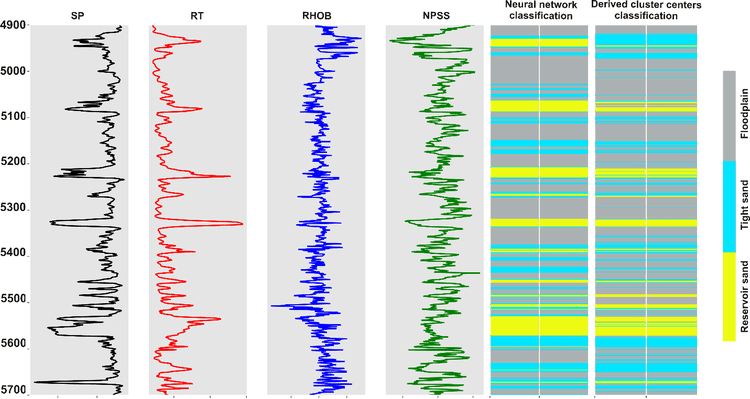
To demonstrate the effectiveness of the proposed machine learning pipeline and the quality of the obtained cluster centers, a lithofacies classification was produced from the derived cluster centers. In the next figure, from left to right, the first four panels show the wireline log data used to train the neural network. The following panel displays the neural network-based lithofacies classification. Note that three lithofacies classes were predicted: reservoir sand (bands in yellow), tight sand (bands in cyan), and floodplain rocks (bands in gray). The last panel displays the lithofacies classification from the derived cluster centers. There is a strong match between the two classifications in terms of the occurrence of reservoir sands, but also in the lithofacies sequence and boundaries. I am thankful to Geophysical Insights to grant the permission to present this research work at the upcoming SEG-SBGf Workshop on Machine Learning.

If you are interested in learning on how we extract meaningful geological information from seismic with machine learning, and how our technology has helped geoscientists in finding hydrocarbons, please visit us at https://www.geoinsights.com/.

Or, if you desire further information, feel free to contact us.