Geobody Interpretation Through Multi-Attribute Surveys, Natural Clusters and Machine Learning

Summary

Multi-attribute seismic samples (even as entire attribute surveys), Principal Component Analysis (PCA), attribute selection lists, and natural clusters in attribute space are candidate inputs to machine learning engines that can operate on these data to train neural network topologies and generate autopicked geobodies. This paper sets out a unified mathematical framework for the process from seismic samples to geobodies. SOM is discussed in the context of inversion as a dimensionality-reducing classifier to deliver a winning neuron set. PCA is a means to more clearly illuminate features of a particular class of geologic geobodies. These principles are demonstrated with geobody autopicking below conventional thin bed resolution on a standard wedge model.

Introduction

Seismic attributes are now an integral component of nearly every 3D seismic interpretation.  Early development in seismic attributes is traced to Taner and Sheriff (1977).  Attributes have a variety of purposes for both general exploration and reservoir characterization, as laid out clearly by Chopra and Marfurt (2007).  Taner (2003) summarizes attribute mathematics with a discussion of usage.

Self-Organizing Maps (SOM) are a type of unsupervised neural networks that self-train in the sense that they obtain information directly from the data.  The SOM neural network is completely self-taught, which is in contrast to the perceptron and its various cousins undergo supervised training.  The winning neuron set that results from training then classifies the training samples to test itself by finding the nearest neuron to each training sample (winning neuron).  In addition, other data may be classified as well.  First discovered by Kohonen (1984), then advanced and expanded by its success in a number of areas (Kohonen, 2001; Laaksonen, 2011), SOM has become a part of several established neural network textbooks, namely Haykin (2009) and Dutta, Hart and Stork (2001).  Although the style of SOM discussed here has been used commercially for several years, only recently have results on conventional DHI plays been published (Roden, Smith and Sacrey, 2015).

Three Spaces

The concept of framing seismic attributes as multi-attribute seismic samples for SOM training and classification was presented by Taner, Treitel, and Smith (2009) in an SEG Workshop.  In that presentation, survey data and their computed attributes reside in survey space.  The neural network resides in neuron topology space.  These two meet in attribute space where neurons hunt for natural clusters and learn their characteristics.

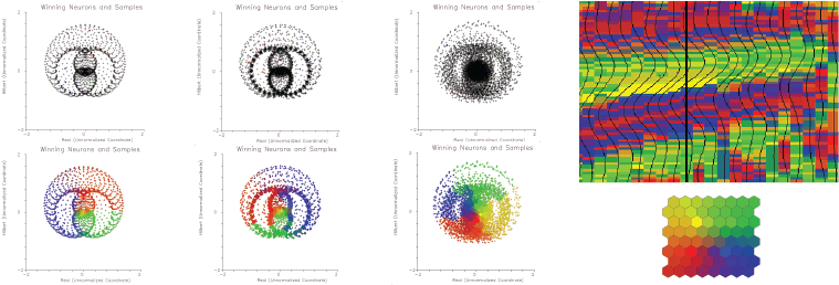
Results were shown for 3D surveys over the venerable Stratton Field and a Gulf of Mexico salt dome.  The Stratton Field SOM results clearly demonstrated that there are continuous geobody events in the weak reflectivity zone between C38 and F11 events, some of which are well below seismic tuning thickness, that could be tied to conventional reflections and which correlated with wireline logs at the wells.  Studies of SOM machine learning of seismic models were presented by Smith and Taner (2010).  They showed how winning neurons distribute themselves in attribute space in proportion to the density of multi-attribute samples.  Finally, interpretation of SOM salt dome results found a low probability zone where multi-attribute samples of poor fit correlated with an apparent salt seal and DHI down-dip conformance (Smith and Treitel, 2010).

Survey Space to Attribute Space:

Ordinary seismic samples of amplitude traces in a 3D survey may be described as an ordered set .  A multi-attribute survey is a “Super 3D Survey” constructed by combining a number of attribute surveys with the amplitude survey.  This adds another dimension to the set and another subscript, so the new set of samples including the additional attributes is .  These data may be thought of as separate surveys or equivalently separate samples within one survey.  Within a single survey, each sample is a multi-attribute vector.  This reduces the subscript by one count so the set of multi-attribute vectors  .

Next, a two-way mapping function may be defined that references the location of any sample in the 3D survey by single and triplet indices Now the three survey coordinates may be gathered into a single index so the multi-attribute vector samples are also an unordered set in attribute space  The index map is a way to find a sample a sample in attribute space from survey space and vice versa.

Multi-attribute sample and set in attribute space:

A multi-attribute seismic sample is a column vector in an ordered set of three subscripts c,d,e representing sample index, trace index, and line index. Survey bins refer to indices d and e.  These samples may also be organized into an unordered set with subscript i.  They are members of an -dimensional real space.  The attribute data are normalized so in fact multi-attribute samples reside in scaled attribute space.

Natural clusters in attribute space:

Just as there are reflecting horizons in survey space, there must be clusters of coherent energy in attribute space.  Random samples, which carry no information, are uniformly distributed in attribute space just as in survey space.  The set  of natural clusters in attribute space is unordered and contains m  members.  Here, the brackets [1, M]  indicate an index range.  The natural clusters may reside anywhere in attribute space, but attribute space is filled with multi-attribute samples, only some of which are meaningful natural clusters.  Natural clusters may be big or small, tightly packed or diffuse.  The rest of the samples are scattered throughout F-space.  Natural clusters are discovered in attribute space with learning machines imbued with simple training rules and aided by properties of their neural networks.

A single natural cluster:

A natural  cluster may have elements in it.  Every natural cluster is expected to have a different number of multi-attribute samples associated with it.  Each element is taken from the pool of the set of all multi-attribute samples   Every natural cluster may have a different number of multi-attribute samples associated with it so for any natural cluster, then N(m).  Every natural cluster has its own unique properties described by the subset of samples  that are associated with it.  Some sample subsets associated with a winning neuron are small (“not so popular”) and some subsets are large (“very popular”).  The distribution of Euclidean distances may be tight (“packed”) or loose (“diffuse”).

Geobody sample and geobody set in survey space:

For this presentation, a geobody G_b is defined as a contiguous region in survey space composed of elements which are identified by members g.  The members of a geobody are an ordered set  which registers with those coordinates of members of the multi-attribute seismic survey .

A geobody member is just an identification number (id), an integer .  Although the 3D seismic survey is a fully populated “brick” with members ,  the geobody members  register at certain contiguous locations, but not all of them.  The geobody  is an amorphous, but contiguous, “blob” within the “brick” of the 3D survey.  The coordinates of the geobody blob in the earth are where  By this, all the multi-attribute samples in the geobody may be found, given the id and three survey coordinates of a seed point.

A single geobody in survey space:
Each geobody is a set of  N geobody members with the same id.  That is, there are N members in , so N(b).  The geobody members for this geobody are taken from the pool of all geobody samples, the set  Some geobodies are small and others large.  Some are tabular, some lenticular, some channels, faults, columns, etc.  So how are geobodies and natural clusters related?

A geobody is not a natural cluster:

This expression is short but sweet.  It says a lot.  On the left is the set of all B geobodies.  On the right is the set of M natural clusters.  The expression says that these two sets aren’t the same.  On the left, the geobody members are id numbers These are in survey space.  On the right, the natural clusters  These are in attribute space.  What this means is that geobodies are not directly revealed by natural clusters.  So, what is missing?

Interpretation is conducted in survey space.  Machine learning is conducted in attribute space.  Someone has to pick the list of attributes.  The attributes must be tailored to the geological question at hand.  And a good geological question is always the best starting point for any interpretation.

A natural cluster is an imaged geobody:
Here, a natural cluster C_m is defined as an unorganized set of two kinds of objects: a function I of a set of geobodies G_i and random noise N.  The number of geobodies is I and unspecified.  The function is an illumination function which places the geobodies in  The illumination function is defined by the choice of attributes.  This is the attribute selection list.  The number of geobodies in a natural cluster C_m is zero or more, 0<i<I.  The geobodies are distributed throughout the 3D survey.

The natural cluster concentrates geobodies of similar illumination properties.  If there are no geobodies or there is no illumination with a particular attribute selection list,  , so the set is only noise.  The attribute selection list is a critically import part of multi-attribute seismic interpretation.  The wrong attribute list may not illuminate any geobodies at all.

Geobody inversion from a math perspective:

Multi-attribute seismic interpretation proceeds from the preceding equation in three parts.  First, as part of an inversion process, a natural cluster   is statistically estimated by a machine learning classifier such as SOM  with a neural network topology.  See Chopra, Castagna and Potniaguie (2006) for a contrasting inversion methodology.  Secondly, SOM employs a simple training rule that a neuron nearest a selected training sample is declared the winner and the winning neuron advances toward the sample a small amount.  Neurons are trained by attraction to samples.  One complete pass through the training samples is called an epoch.  Other machine learning algorithm have other training rules to adapt to data.  Finally, SOM has a dimensionality reducing feature because information contained in natural clusters is transferred (imperfectly) to the winning neuron set in the finalized neural network topology through cooperative learning.  Neurons in winning neuron neighborhood topology move along with the winning neuron in attribute space.  SOM training is also dynamic in that the size of the neighborhood decreases with each training time step so that eventually the neighborhood shrinks so that all subsequent training steps are competitive.

Because is a statistical estimate, let it be called the statistical estimate of the “signal” part of .  The true geobody is independent of an illumination function.  The dimensionality reduction  associated with multi-attribute interpretation has a purpose of geobody recognition through identification, dimensionality reduction and classification.  In fact, in the chain of steps there is a mapping and un-mapping process with no guarantee that the geobody will be recovered:

However, the image function   may be inappropriate to illuminate the geobody in F-space because of a poor choice of attributes.  So at best, the geobodies is illuminated by an imperfect set of attributes and detected by a classifier that is primitive.  The results often must be combined, edited and packaged into useful, interpreted geobody units, ready to be incorporated into an evolving geomodel on which the interpretation will rest.

Attribute Space Illumination

One fundamental aspect of machine learning is dimensionality reduction from attribute space because its dimensions are usually beyond our grasp.  The approach taken here is from the perspective of manifolds which are defined as spaces with the property of “mapability” where Euclidean coordinates may be safely employed within any local neighborhood (Haykin, 2009, p.437-442).

The manifold assumption is important because SOM learning is routinely conducted on multi-attribute samples in attribute space using Euclidean distances to move neurons during training.  One of the first concerns of dimensionality reduction is the potential to lose details in natural clusters.  In practice, it has been found that halving the original amplitude sample interval is advantageous, but further downsampling has not proven to be beneficial.  Infilling a natural cluster allows neurons during competitive training to adapt to subtle details that might be missed in the original data.

Curse of Dimensionality

The Curse of Dimensionality (Haykin, 2009) is, in fact, many curses.  One problem is that uniformly sampled space increases dramatically with increasing dimensionality.  This has implications when gathering training samples for a neural network.  For example, cutting a unit length bar (1-D) with a sample interval of .01 results in 100 samples.  Dividing a unit length hypercube in 10-D with a similar sample interval results in 10²⁰ samples (10¹⁰ x 10²).  If the nature of attribute space requires uniform sampling across a broad numerical range, then a large number of attributes may not be practical.  However, uniform sampling is not an issue here because the objective is to locate and detail features of natural clusters.

Also, not all attributes are important.  In the hunt for natural clusters, PCA (Haykin, 2009) is often a valuable tool to assess the relative merits of each attribute in a SOM attribute selection list.  Depending on geologic objectives, several dominant attributes may be picked from the first, second or even third principal eigenvectors or may pick all attributes from one principle eigenvector.

Geobody inversion from an interpretation perspective:

Multi-attribute seismic interpretation is finding geobodies in survey space aided by machine learning tools that hunt for natural clusters in attribute space.  The interpreter’s critical role in this process is the following:

• Choose questions that carry exploration toward meaningful conclusions.
• Be creative with seismic attributes so as to effectively address illumination of geologic geobodies.
• Pick attribute selection lists with the assistance of PCA.
• Review the results of machine learning which may identify interesting geobodies  in natural clusters autopicked by SOM.
• Look through the noise to edit and build geobodies  with a workbench of visualization displays and a variety of statistical decision-making tools.
• Construct geomodels by combining autopicked geobodies which in turn allow predictions on where to make better drilling decisions.

The Geomodel

After classification, picking geobodies from their winning neurons starts by filling an empty geomodel .  Natural clusters are consolidators of geobodies with common properties in attribute space so M < B.  In fact, it is often found that M << B .  That is, geobodies “stack” in attribute space.  Seismic data is noisy.  Natural clusters are consequentially statistical.  Not every sample g classified by a winning neuron is important although SOM classifies every sample. Samples that are a poor fit are probably noise.  Construction of a sensible geomodel depends on answering well thought out geological questions and phrased by selection of appropriate attribute selection lists.

Working below classic seismic tuning thickness

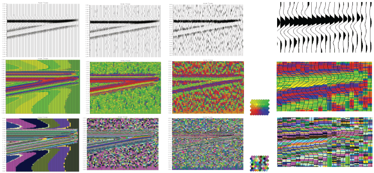
Classical seismic tuning thickness is λ/4.  Combining vertical incidence layer thickness  with  λ=V/f leads to a critical layer thickness  Resolution below classical seismic tuning thickness has been demonstrated with multi-attribute seismic samples and a machine learning classifier operating on those samples in scaled attribute space (Roden, et. al., 2015). High-quality natural clusters in attribute space imply tight, dense balls (low entropy, high density).  SOM training and classification of a classical wedge model at three noise levels is shown in Figures 1 and 2 which show tracking well below tuning thickness.

Seismic Processing: Processing the survey at a fine sample interval is preferred over resampling the final survey to a fine sample interval. Highest S/N ratio is always preferred. Preprocessing: Fine sample interval of base survey is preferred to raising the density of natural clusters and then computing attributes, but do not compute attributes and then resample because some attributes are not continuous functions. Derive all attributes from a single base survey in order to avoid misties. Attribute Selection List: Prefer attributes that address the specific properties of an intended geologic geobody. Working below tuning, prefer instantaneous attributes over attributes requiring spatial sampling.  Thin bed results on 3D surveys in the Eagle Ford Shale Facies of South Texas and in the Alibel horizon of the Middle Frio Onshore Texas and Group corroborated with extensive well control to verify consistent results for more accurate mapping of facies below tuning without usual traditional frequency assumptions (Roden, Smith, Santogrossi and Sacrey, personal communication, 2017).

Conclusion

There is a firm mathematical basis for a unified treatment of multi-attribute seismic samples, natural clusters, geobodies and machine learning classifiers such as SOM.  Interpretation of multi-attribute seismic data is showing great promise, having demonstrated resolution well below conventional seismic thin bed resolution due to high-quality natural clusters in attribute space which have been detected by a robust classifier such as SOM.

Acknowledgments

I am thankful to have worked with two great geoscientists, Tury Taner and Sven Treitel during the genesis of these ideas.  I am also grateful to work with an inspired and inspiring team of coworkers who are equally committed to excellence.  In particular, Rocky Roden and Deborah Sacrey are longstanding associates with a shared curiosity to understand things and colleagues of a hunter’s spirit.

References

Chopra, S. J. Castagna and O. Potniaguine, 2006, Thin-bed reflectivity inversion, Extended abstracts, SEG Annual Meeting, New Orleans.
Chopra, S. and K.J. Marfurt, 2007, Seismic attributes for prospect identification and reservoir characterization, Geophysical Developments No. 11, SEG.
Dutta, R.O., P.E. Hart and D.G. Stork, 2001, Pattern Classification, 2nd ed.: Wiley.
Haykin, S., 2009, Neural networks and learning machines, 3rd ed.: Pearson.
Kohonen, T., 1984, Self-organization and associative memory, pp 125-245. Springer-Verlag. Berlin.
Kohonen, T., 2001, Self-organizing maps: Third extended addition, Springer, Series in Information Services.
Laaksonen, J. and T. Honkela, 2011, Advances in self-organizing maps, 8th International Workshop, WSOM 2011 Espoo, Finland, Springer.
Ma, Y. and Y. Fu, 2012, Manifold Learning Theory and Applications, CRC Press, Boca Raton.
Roden, R., T. Smith and D. Sacrey, 2015, Geologic pattern recognition from seismic attributes, principal component analysis and self-organizing maps, Interpretation, SEG, November 2015, SAE59-83.
Smith, T., and M.T. Taner, 2010, Natural clusters in multi-attribute seismics found with self-organizing maps: Source and signal processing section paper 5: Presented at Robinson-Treitel Spring Symposium by GSH/SEG, Extended Abstracts.
Smith, T. and S. Treitel, 2010, Self-organizing artificial neural nets for automatic anomaly identification, Expanded abstracts, SEG Annual Convention, Denver.
Taner, M.T., 2003, Attributes revisited, http://www.rocksolidimages.com/attributes-revisited/, accessed 22 March 2017.
Taner, M.T., and R.E. Sheriff, 1977, Application of amplitude, frequency, and other attributes, to stratigraphic and hydrocarbon determination, in C.E. Payton, ed., Applications to hydrocarbon exploration: AAPG Memoir 26, 301–327.
Taner, M.T., S. Treitel, and T. Smith, 2009, Self-organizing maps of multi-attribute 3D seismic reflection surveys, Presented at the 79th International SEG Convention, SEG 2009 Workshop on “What’s New in Seismic Interpretation,” Paper no. 6.