By Bob Hardage, Tom Smith, Diana Sava, Yi Wang, Rocky Roden, Gary Jones, and Sarah Stanley | Published with permission: Interpretation Journal | November 2020
Table of contents
-
Abstract
-
Introduction
-
Study Area
-
Log data spanning the Wolfberry interval
-
Equivalence of P-SV and SV-P imaging
-
Examples of P-P and SV-P profiles across the study area
-
Interpreting P-P and SV-P images with ML software
-
Step 1 — PCA (determining the relative importance of seismic attributes)
-
Comparison of P-P and S-mode principal components
-
Step 2 — Displaying principal component information (profile views)
-
Step 3 — Displaying principal component information (map views)
-
Why do Wolfberry P-P and SV-P images differ?
-
Conclusions
-
Acknowledgments
-
Data and materials availability
Abstract
The Permian Basin of west Texas spans two major subbasins — the Midland Basin and the Delaware Basin. Both basins contain Wolfcampian- to Leonardian-age turbidites that form thick sections of prolific unconventional reservoirs. For the past several years, the most active drilling targets in the United States have been the Wolfberry turbidite interval of the Midland Basin and the Wolfbone turbidite interval in the Delaware Basin. We have used two new technologies to examine the internal architecture and fabric of a thick interval of these unconventional drilling targets with seismic reflection seismology. First, we used seismic interpretation software that uses unsupervised machine learning (ML), so that a higher level of detail could be extracted from seismic images. Second, we complemented our P-P imaging of Wolfberry turbidites with a new seismic imaging option, that being SV-P (or converted-P) imaging. Because vertical vibrators, particularly arrays of vertical vibrators, produce downgoing P and downgoing SV illuminating wavefields, SV-P reflections can usually be extracted from the same vertical-geophone responses as are P-P reflections. The combination of these two images essentially doubles the amount of information that can be extracted from data generated by P sources and recorded with vertical geophones. SV-P imaging with P sources has been ignored by reflection seismologists for decades, so we felt an obligation to illustrate the value of this ignored seismic mode. These two new tools — SV-P imaging and interpreting P-P and SV-P images via unsupervised ML — expanded our insights into the internal architecture and fabric of Wolfberry turbidites. Our work provides interpreters a much-needed example of applying unsupervised ML technology in a joint interpretation of P- and S-wave data.
Introduction
Thirteen-year-old legacy 3D 3C seismic data acquired on the western shelf of the Midland Basin, where there is a thick stack of Wolfberry turbidites, were used in this study, so these unconventional reservoirs could be
investigated with P-wave and S-wave seismic attributes. Wolfberry turbidites form a high-interest drilling target of unconventional reservoirs that extend upward from the Wolfcamp (Wolf) formation to the Sprayberry (berry) formation. This Wolfberry interval of stacked turbidite flows is approximately 3000 ft (1000 m) thick across our study area.
Three-dimensional P-P, P-SV, and SV-P data volumes were interpreted with commercial software that uses unsupervised machine learning (ML) principles. Interpretation focused on determining if combinations of seismic attributes extracted through joint interpretations of depth-equivalent P-mode and S-mode data provide improved understanding of the internal architecture and fabric of turbidite assemblages. This approach allowed specific P-wave and S-wave geobodies embedded in stacked turbidites to be isolated.
Mineral counts based on analyses of thin sections cut from Wolfberry cores allowed us to propose the hypothesis that these seismic geobodies represent spatial distributions of distinct mineral mixtures found in matrices of Wolfberry turbidite units. Turbidite matrices that have different mineral mixtures have different stiffness coefficients. Turbidite matrix-fabric 1 thus creates P and S reflection wavelets that have different attributes and/or different numerical ranges of attributes than does turbidite matrix-fabric 2. Each searching neuron that migrates through each P and S attribute space in unsupervised ML searches identifies the x-y-z coordinates where specific combinations of seismic attributes and specific numerical ranges of those attributes exist. Maps of these data coordinates describe a geobody. We thus view a geobody created in this study as a region inside a turbidite assemblage that has a distinct rock fabric. This fabric may be associated with a single turbidite, it may be only a portion of a single turbidite, or it may span a group of several individual turbidites.
SV-P (converted-P) data provided insights into the internal architecture and fabric of turbidites that were equal to, and sometimes better than, insights provided by P-P and P-SV data. The SV-P data used in this study were generated by a traditional P source (an array of three inline vertical vibrators) and were recorded with vertical geophones. Because these 3D seismic data were acquired 13 years before this study was done, this project demonstrates that SV-P data can be extracted from hundreds of thousands of square kilometers of legacy seismic data generated by P sources and recorded with vertical geophones. Such P source vertical-geophone data are preserved in many digital data libraries around the globe. There are, in fact, several thousands of square kilometers of legacy P source vertical-geophone seismic data across the Permian Basin alone.
Study Area
Our study area is shown in Figure 1. Data were generated by an inline array of three vertical vibrators that occupied a grid of source stations distributed across a 3 × 3 mi area of surface-source illumination. Data were recorded by a 2 × 2 mi grid of 3C geophones centered inside this source-station grid. The map scale used for Figure 1 would cause this seismic grid to appear as only a small dot on this basin-view map.
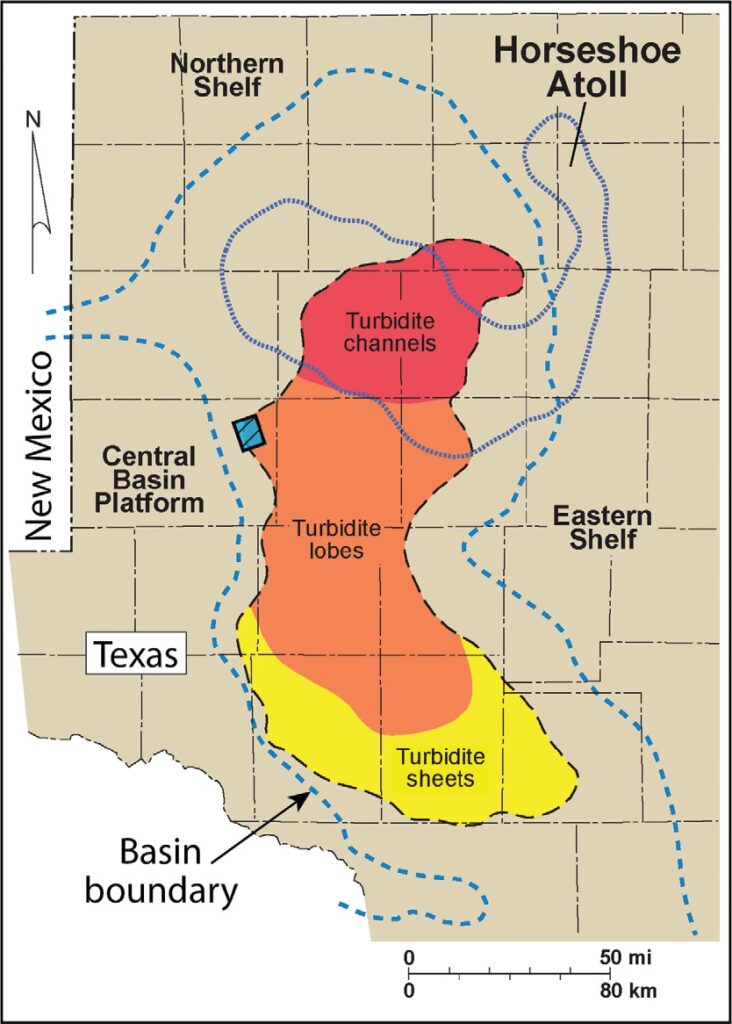
An objective of this paper is to illustrate that this new concept of extracting SV-P images from vertical-geophone data can be included in seismic interpretation studies across other areas where P source, vertical-geophone, legacy seismic surveys are available. Because data used in this study were recorded with 3C geophones, horizontal-geophone data could have been processed to extract S-S reflections generated by the direct S illuminating wavefields produced by the P source (three inline vertical vibrators). In fact, a brute stack of S-S data was constructed and was of an acceptable quality for a brute stack. However, because only a limited amount of 3C geophone data exist across most turbidite prospect areas, S-S data processing efforts were set aside to concentrate fully on demonstrating the value of SV-P modes that can be extracted from traditional vertical-geophone data. There are huge amounts of legacy vertical-geophone data across the Permian Basin and other basins that will allow SV-P studies of other turbidite systems, or of any deep geologic targets, to be repeated by other investigators.
Log data spanning the Wolfberry interval
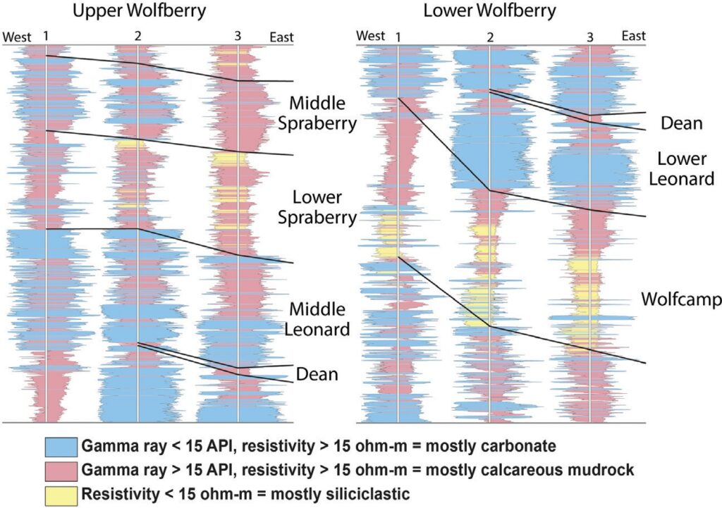
After examining many thin sections extracted from cores in logged wells, Hamlin
and Baumgardner (2012) in their seminal report for the Texas Bureau of Economic Geology conclude that the mineralogical complexity present in Wolfberry turbidites could be reasonably represented by the three-color rock-facies distinctions used in Figure 2. These three general facies classifications of Wolfberry turbidites were then related to gamma-ray and resistivity log readings. In Figure 2,the left-side boundary of each colored turbidite-facies column indicates gamma-ray readings and the right-side boundary indicates resistivity-log values. An examination of these log responses and their simplified lithofacies interpretations will help investigators understand the thicknesses, lateral dimensions, areal shapes, and internal mineralogical frameworks of Wolfberry turbidites. The voluminous report by Hamlin
and Baumgardner (2012) shows that Wolfberry turbidite shapes, sizes, thicknesses, and mineralogical content vary rapidly in the vertical and horizontal directions across the Midland Basin. One should thus expect that most seismic reflections across Wolfberry turbidite intervals will be continuous for only short distances. Seismic interpreters should thus assume that age-equivalent turbidite units will be difficult to define with seismic data.
Equivalence of P-SV and SV-P imaging
One objective of this study was to include S-mode imaging in the study of Wolfberry turbidites. Data acquired in a legacy P source 3D 3C seismic survey were used so that the P-P and P-SV data could be used in a joint interpretation of Wolfberry turbidite targets inside the small area spanned by this seismic grid. Unfortunately, P-SV data generated in this legacy seismic survey have a prominent acquisition footprint. The companion P-P image showed no hint of an acquisition footprint. This P-SV acquisition footprint caused our investigation to switch to SV-P data as a substitute for P-SV data. When stratigraphic layering is approximately horizontal and lateral changes in P and S velocities are not excessive, the P-SV and SV-P images should be identical.
SV-P data extracted from the vertical geophone data contained no evidence of an acquisition footprint. In PSV imaging that uses data generated at source station A and recorded at geophone station B, the P-SV image point is closer to receiver station B than it is to source station A. In contrast, the SV-P reflection point for this same source-receiver pair is closer to source station A than to receiver station B. This distinction in the spatial distributions of P-SV and SV-P image points evidently can cause one converted mode (P-SV in this case) to have an acquisition footprint, but its companion conversion mode (SV-P in this case) to not have an acquisition footprint. People who design 3D 3C seismic acquisition programs need to be sensitive to this possibility and ensure that there is a degree of randomness in the spacings between adjacent source stations and/or receiver stations. Random station spacings tend to eliminate acquisition footprints.
P-SV and SV-P images should be identical in that part of the seismic image space where the P-SV and SV-P image points overlay each other. This principle has been established by Aki and Richards (1980, 2002) who develop the following equation:
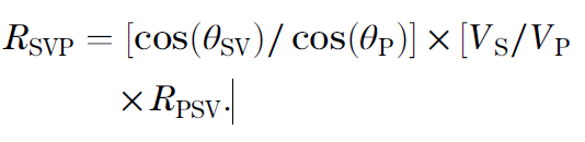
In this equation, RSVP is the SV-P reflection coefficient at a targeted interface, RPSV is the P-SV reflection coefficient at that same interface, .SV is the incident angle of the downgoing SV ray-path, .P is the reflected angle of the up-going P raypath, and VS and VP are, respectively, the S-wave velocity and P-wave velocity in the medium above the interface. This equation shows that RSVP and RPSV have the same algebraic sign at a reflecting interface and, because of the numerical balancing effect of the angle and velocity terms in equation 1, the magnitude of RSVP should usually be slightly less than the magnitude of RPSV at that interface.
The principle that SV-P and P-SV images are identical was demonstrated with real 2D 9C data by Frasier and Winterstein (1990). The downgoing SV wavefield used to construct the SV-P data in their award-winning 1990 publication was generated by a horizontal vibrator. In contrast, the downgoing SV wavefields used to generate SV-P data across Wolfberry turbidites in this study were generated by an array of three inline vertical vibrators. Presently, the SV-P image illustrated in Frasier and Winterstein’s (1990) paper is considered to not only be the first, but also to be the only, published example of an SV-P image in geophysical literature. Researchers at the Bureau of Economic Geology, the University of Texas at Austin, began providing the sponsors of their research consortium private examples of SV-P images made with P sources and recorded with vertical geophones in 2009 and then began revealing several years of SV-P research in open publications in 2014 (Hardage et al., 2014; Hardage and Wagner, 2014a,2014b; Li and Hardage, 2015; Hardage, 2017a, 2017b, 2017c, 2017d; Karr, 2017; Li, et al., 2017; Wagner and Hardage, 2017; Gupta and Hardage, 2017; Hardage and Wagner, 2018a, 2018b). Presently, there are no published works by other investigators on the topic of practicing S-wave reflection seismology with data generated by P sources and recorded by vertical geophones.
Examples of P-P and SV-P profiles across the study area
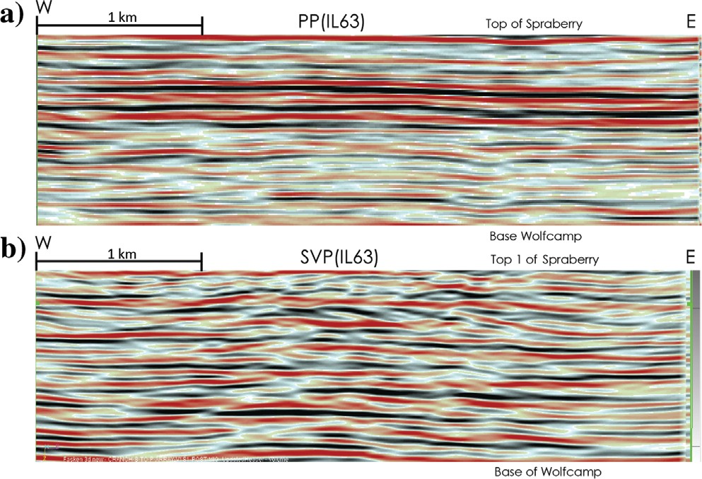
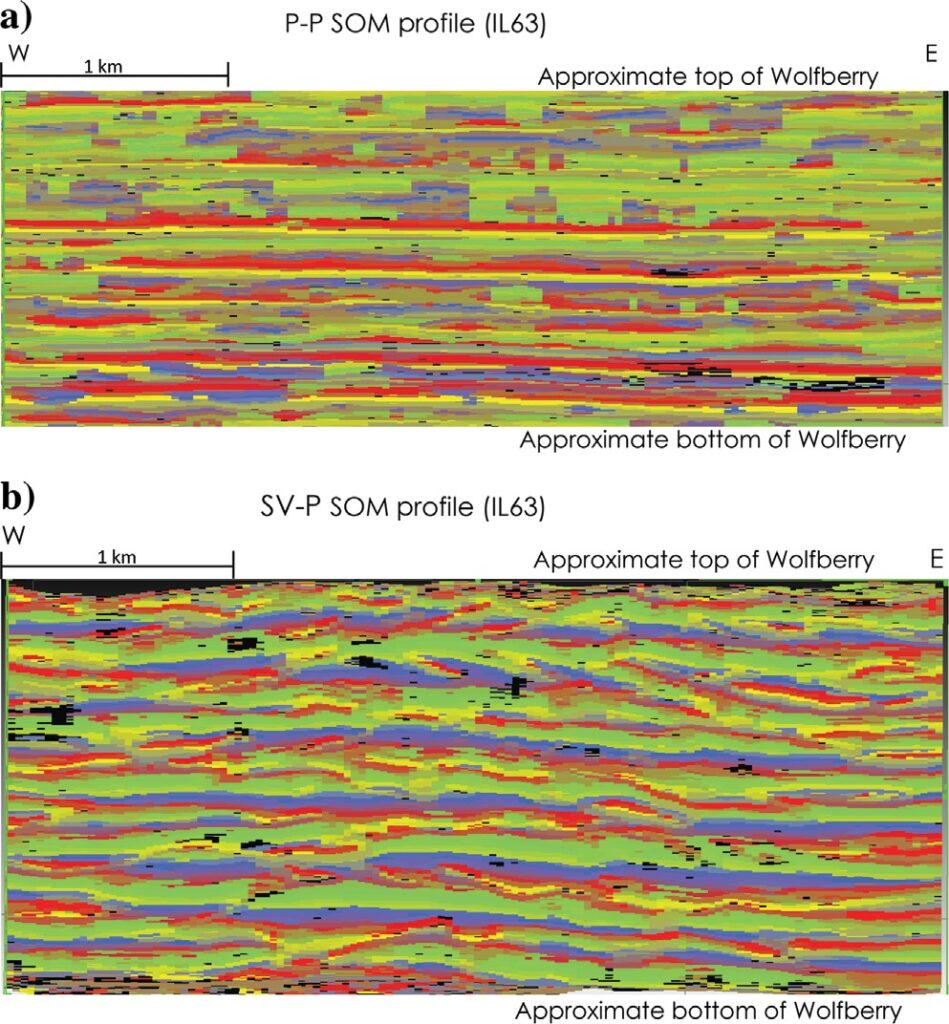
Examples of west-to-east P-P and SV-P profiles passing through the approximate center of the 3D seismic image space used in this study are shown in Figure 3.
The same coordinate profile through the companion P-SV data volume is not shown because the acquisition footprint embedded in the P-SV data volume makes those data unsuitable for analysis. This P-SV acquisition footprint will be shown later in map views of the P-P, P-SV, and SV-P amplitude behaviors.
The vertical coordinates of these P-P and SV-P profiles start slightly above the top of the Sprayberry and extend slightly deeper than the base of the Wolfcamp. The entire Wolfberry interval of stacked turbidites is thus shown in each profile. The vertical and horizontal axes are not labeled to protect the operational activity of the data owner. Figure 1
shows that the east–west San Simon Channel enters the Midland Basin a short distance northwest of our study area. As a result, some turbidite sediment inflow can be from the west and northwest at our location on the western shelf of the Midland Basin. If any inflow has a westward component, some turbidites should progress from left to right across the seismic profiles in Figure 3. The Midland Basin deepens significantly to the east, and the Wolfberry turbidite interval thickens as gravity-driven flows of sediment from the north and from the western shelf fill this deeper basin area. As shown in Figure 3, SV-P data show more evidence of stacked, downlapping units like one would expect to see in gravity-driven sediment movement than do P-P data.
Interpreting P-P and SV-P images with ML software
ML is arguably the most important technology presently being introduced into the seismic interpretation community. The first ML procedure used in this study was to determine what types of seismic information should be focused on as P-P and SV-P images of Wolf-berry turbidites are interpreted. This goal was accomplished by applying a principal component analysis (PCA) to combinations of trial attributes extracted first from the P-P image, and then from the SV-P image, to determine the ranked order of importance of information provided by selected seismic attributes in each image space. In this methodology, each image space describes the value of one specific seismic attribute at each data point in the 3D image space. There is an image space for each seismic attribute that is applied to the P-P data volume and an image space for each attribute calculated for the SV-P data volume.
The second procedure was to visualize where specific combinations of these critical information-bearing attributes were positioned in the P-P and SV-P seismic-survey space. This visualization objective was achieved by constructing self-organized maps (SOMs) that show image coordinates where distinct-color neurons found clusters of specific combinations of seismic attributes. A description of PCA and SOM seismic procedures and applications has been published by Roden et al. (2015).
Step 1 — PCA (determining the relative importance of seismic attributes)
Fifteen instantaneous seismic attributes that are helpful for defining information content in P-P data were calculated throughout that part of the 3D image space occupied by Wolfberry turbidites. Following these calculations, P-P data then existed not only in their traditional 3D, x-y-z, seismic-survey space that interpreters have used for decades, but they also existed in 15 3D, x-y-z, instantaneous-attribute spaces, each of which is also an image of the Wolfberry turbidite system. Collectively, these P-P data and their 15 instantaneous attributes form a 16D P-P attribute space, and each data point inside the Wolfberry turbidite interval has 16 P-P attribute values.
These same 15 instantaneous seismic attributes were then calculated throughout that part of the 3D SV-P data space that encapsulated the same Wolfberry turbidites. SV-P data then existed in the traditional 3D x-y-z seismic survey space and also in fifteen 3D x-y-z instantaneous seismic-attribute spaces, which created a set of 16 SV-P attribute volumes spanning the Wolfberry turbidites.
A PCA was applied to the suite of 16 P-P attribute spaces to create the P-P principal components (sometimes abbreviated as PCs) that, collectively, defined the relative importance of attribute information embedded in the P-P Wolfberry turbidite images. A similar procedure was then applied to the 16 SV-P attribute spaces to create a second suite of PCs that, collectively, defined the relative importance of attribute information embedded in the SV-P Wolfberry turbidite images.
An important ML axiom is “if data consist of N observations that have M variations, then the number of principal components required to describe the data is min{[N-1], M}.” In this study, N would be the several thousands of data points in the P-P image space (or in the SV-P image space) and M would be the 16 attributes selected to describe the information embedded in the P-P data (and also in the SV-P data). The number of principal components that needed to be calculated to properly apply unsupervised ML to either our P-P data, or to our SV-P data, was thus 16.
For this study, a PCA of our Wolfberry P-P data required that a 16D ellipsoid be fitted to the 16D P-P seismic-attribute space. Because attributes have different units and ranges of value (e.g., frequency units versus phase units; acceleration range versus envelope-slope range), each attribute distribution is normalized so that it has zero mean and unit variance. By doing this normalization, no one attribute is statistically more important than any other. All possible combinations of pairs of attributes can then be compared for their relative importance using a simple sample-to-sample multiplication and summation — i.e., a zero-lag correlation.
The first 16D principal component (PC1) is a vector from the PCA that points in the direction where the variance of all pairs of these normalized attributes is a maximum. Variance in normalized attributes is analogous to the “amount of information.” An attribute with a large variance provides a large amount of information. If an attribute has no variance, it is a constant value and provides no information. PC1 thus describes the largest possible amount of information in the 16D P-P attribute data. The second 16D principal component (PC2) accounts for the second largest variance (the second largest amount of information) in 16D P-P attribute data that is orthogonal to PC1, PC3 accounts for the third largest variance in 16D P-P attribute data that is orthogonal to PC1 and PC2, and so forth until the last principal component (PC16) is considered. PC16 accounts for the direction in 16D P-P attribute data that has the least variance and that is orthogonal to all 15 previously calculated PCs. This PCA procedure was then repeated with the 16 SV-P attribute volumes to determine the 16 PCs that collectively describe the ranked order of importance of attribute information embedded in our SV-P image of Wolfberry turbidites.
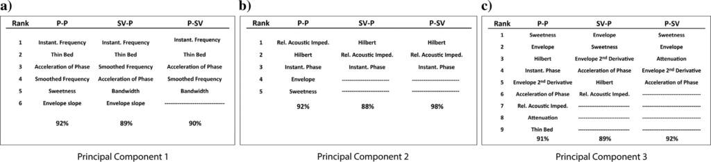
Figure 4 illustrates the rank order in which seismic attributes contributed information to the first three P-P, SV-P, and P-SV principal components. The construction of each PC was stopped, arbitrarily, when the information content in the sequence of PCs built to approximately 90% of the total amount of available information that existed in the 16D attribute space. Interpreters use different criteria to decide how many PCs should be used in an ML interpretation. For example, some interpreters use only the first three PCs regardless of the amount of information that is provided by those three PCs. Even with ML technology, seismic interpretation will, and should, be practiced differently by different people.
The percent of total available information carried by each principal component in Figure 4 is indicated by the percentage number written below each instantaneous-attribute list. Even though P-SV data were not used for interpretation purposes because the data were contaminated by an acquisition footprint, P-SV data are included in this attribute list to understand which seismic attributes provide significant amounts of P-SV information.
Readers should examine the list of attributes that builds PC1 for P-P data in Figure 4a, then the list of P-P attributes that builds PC2 in Figure 4b, and then the P-P list that builds PC3 in Figure 4c to see that a high-rank P-P seismic attribute in one P-P principal component rarely appears in a high-rank position in another P-P principal component. This outcome occurs because PC1 points in the direction of maximum information, PC2 points in the direction of second-most maximum information, and PC3 points in the direction of third-most maximum information. High-rank PCs thus capture huge chunks of the most critical attributes, leaving only small amounts of these key attributes to be used by lower rank PCs. This same observation also applies to the SV-P and P-SV principal components in Figure 4a–4c.
The first 9 principal components (of the 16 possible PCs) captured approximately 90%, or more, of the total information embedded in the P-P and SV-P data (Figure 5). Thus, only the first 9 PCs extracted from the P-P Wolfberry turbidite data, and likewise only the first 9 PCs extracted from the SV-P data, were used in unsupervised ML analyses. This choice to ensure that 90% of the information embedded in P-P and SV-P images of Wolfberry turbidites would be used was strictly an arbitrary decision. A 70% or 80% level of information can often be sufficient to illustrate critical geologic features.
Comparison of P-P and S-mode principal components
Because this study uses unsupervised ML concepts in a joint interpretation of P-wave and S-wave images, it is important to compare principal components deter- mined from companion P-P, SV-P, and P-SV data volumes. The objective of this comparison is to define which seismic attributes make major contributions to the first two or three principal components of P-P data and then determine if these same attributes make significant contributions to the first two or three principal components of S-mode data. By understanding which seismic attributes build the most dominant P and S principal components, interpreters will know if P-P data and S-mode data are affected in approximately the same way by the same seismic attributes, or if the attributes that influence S-mode data are significantly different from the attributes that influence P-P data.
The information in Figure 4 allows this type of investigation to be done. Figure 4a shows that the first four attributes that contribute to the first principal component of P-P, SV-P, and P-SV data are identical and are essentially in the same ranked order of contribution. Likewise, the first three ranked attributes that contribute information to the second P-P, SV-P, and P-SV principal component are identical, and they are essentially in the same ranked order. This consistency continues into principal component 3, where the first two ranked attributes of the third P-P, SV-P, and P-SV principal component are identical.
At least two important conclusions can be made
from these results. First, the acquisition footprint em- bedded in the P-SV data does not cause P-SV principal components to have a dramatically different information structure than the information structure contained in the PCs of P-P and SV-P data, which have no acquisition footprint. PCA results in the Wolfberry P-SV image space are not significantly different from PCAs in the P-P and SV-P image spaces. This observation leads to the conclusion that, in this case, P-SV attributes were not affected by the P-SV acquisition footprint. One should not assume, however, that attributes of a seismic wave mode will always remain stable inside and outside of acquisition-footprint areas.
Second, and probably more important, is the fact that P-P data are not influenced by a different set of seismic attributes than are SV-P converted-mode data. Our P and S data are, to first-order accuracy, influenced by the same seismic attributes in approximately the same ranked order of influence. A factor that may need to be considered is that the P and S modes used in this study were generated by the same source — an inline array of three vertical vibrators — at the same instant of clock time and at exactly the same surface coordinates. To carry forward this significant observation, a PCA now needs to be applied to 3C data where the P-P mode is generated by a vertical vibrator but the S-wave data are generated by a different source — perhaps a horizontal vibrator — at a different clock time (perhaps even on a different day) and at surface coordinates that are slightly displaced, perhaps by only 2 or 3 m, from the P-source position. Other questions can also be considered, such as, is the finding that the rank order of attributes that influence P data is identical to the rank order of attributes that influence S data an outcome that is unique to this particular seismic survey, or to the particular data window that was analyzed, or to the type of rocks that were imaged? This early effort to compare the seismic-attribute structure of P and S data is placed in the public domain for others to expand on and to address questions of this nature.
Step 2 — Displaying principal component information (profile views)
To use principal component information, it is essential to implement a procedure that takes advantage of multiple coincident attributes in an attribute space that constitutes a common-image space. The first advantage of implementing this procedure is the dimensionality reduction afforded by a PCA analysis. The list of 16 “trial attributes” used in this study was reduced by interpreting our PCA analysis and selecting a shorter list of nine “important attributes” (Figure 5). One may compute a new set of attributes based on just these nine important attributes, and a second PCA analysis of this reduced number of attributes can then be made if desired (Guo, et al., 2009; Brito, 2010; Chopra and Marfurt, 2014). A second set of important attributes can then be computed from the PCs of the first important-attribute set. An alternative is to select the important attributes from the first PCA analysis for further study.
PCA is a linear process and is a suspect procedure if input data themselves are not linearly related. Nonlinear properties do exist among seismic attributes because some attributes are quite different from others. A nonlinear extension of PCA for seismic interpretation shows promise. Although PCA is suitable for dimensionality reduction from a long list of “trial attributes” to a shorter list of “important attributes,” the reduced attribute dimension that results may still be too large for practical seismic interpretation. Each seismic image space is an image of only a single attribute, so many important relationships between attributes are difficult to recognize in a 9D attribute space, or in any attribute space with a dimensionality greater than 3. What is needed is a simultaneous analysis of all attributes (nine attributes in our case). Such simultaneous analyses are possible because of the spatial coincidence of all attribute images.
There is a nonlinear ML technology that reduces attribute dimensionality from the “important attribute” level (nine dimensions in our case) to only two dimensions. This technique is called the self-organizing map (SOM) (Kohonen, 2001; Bishop, 2006; Haykin, 2009; Wilmott, 2019). SOM is a type of ML that preserves clusters of natural information density as a 2D SOM and simultaneously preserves each natural cluster of information in its input attribute dimensions (Haykin, 2009, p. 442–445). A 2D SOM thus contains self-organization properties that allow geologic features embedded in the dimensions of “important” seismic attributes to be displayed and examined.
Some ML algorithms, such as deep learning, are based on an attractive property that an algorithm trains on input training data so that the characteristics of these training data are preserved. Such algorithms are self-adapting. SOM, in contrast, offers an ML property in which regions of information in several reduced dimensions reflect similar regions of information in the original dimensions. Such algorithms are self-organizing, a property that is quite advantageous for seismic interpretation.
SOM ML identifies and preserves information through a network of neurons that learn characteristics of seismic data through simple training rules. In SOM procedures, training rules are refined as one training step follows another. The network itself is a 2D mesh, and the training rules define how information is shared between neurons. In seismic interpretation, training samples are usually constrained to be between two stratigraphic horizons, and each sample is a multi-attribute vector. The volume of training samples is generally confined to a specific region of interpretation interest.
When a SOM procedure is used, ML is, by definition, unsupervised learning because none of the training samples in the region of interest have classification labels. A complete set of classification labels (i.e., winning neuron numbers) are developed by the SOM process. A P-P SOM is created by neurons that have searched through P-P attribute spaces to find natural clusters of multi-attribute data samples. When all neuron training ends, each training sample is associated with one of the neurons in this SOM. After machine training, the neurons have stopped their searching and the result is called the winning neuron set. After training, each seismic sample has a winning neuron. In other words, each seismic sample has been classified. For example, if the SOM is an 8 × 8 network of neurons like we used, each seismic sample has been classified as one of the 64 possible winning neurons. These SOM classifications constitute a new seismic image based on classification numbers.
The principal reason why these SOM procedures are so valuable is that they reduce ML results from the multidimensional attribute space (a 9D space in our example) to a simpler 2D color grid that allows interpreters to see how attribute information is distributed in P-P and SV-P data spaces. The number of cells in this 2D color grid and the distribution of colors among these grid cells are defined by the person interpreting the seismic data. Interpreters should experiment with different magnitudes of neuron populations, ranging from a small population (maybe a 5 × 5 grid), to a medium-size population (perhaps an 8 × 8 grid), to a large population (maybe a 10 × 10 grid). An interpreter can then view each neuron population with different color maps and decide which color depiction of which neuron population best illustrates what they want to see.
One SOM procedure was used to visualize, through classification, where unsupervised ML positioned various classified samples of Wolfberry P-P attributes in the P-P multi-attribute space. A second SOM procedure was used to visualize where unsupervised ML placed various classified samples of Wolfberry SV-P attributes in the SV-P multi-attribute space. The resulting P-P and SV-P classification images that we show in this paper thus display natural clusters of attributes identified by unsupervised ML in the multi-attribute space.
Vertical profiles of SOM results through the central part of P-P and SV-P attribute spaces are displayed as Figure 6. The 2D SOM displays of the 64 colored neurons used to construct each of these profiles are shown later. These SOM vertical profiles are the same profiles shown in Figure 3 that use a traditional linear color scale. Details about the internal architecture and fabric of stacked Wolfberry turbidites are better expressed by the SOM displays in Figure 6, particularly by the SV-P profile, than by traditional color displays. In particular, the SV-P color section has more discontinuous, hummocky events expected of a thick stack of turbidites than do the flatter, smoother events in the P-P color section.
Step 3 — Displaying principal component information (map views)
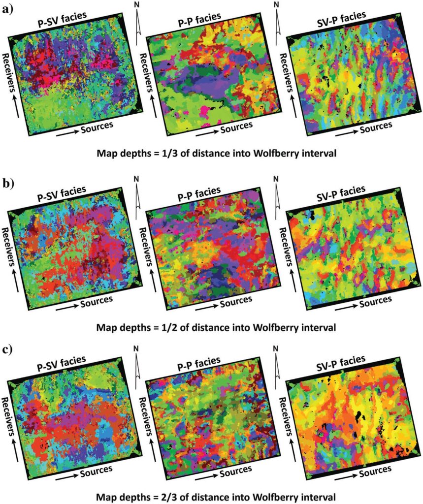
It is particularly informative to view SOM volumes of Wolfberry turbidites in map view. Examples of horizontal slices through P-SV, P-P, and SV-P SOM volumes are displayed in Figure 7. The color at any x-y coordinate in these maps defines which of the winning neurons identified in the SOM displays resides at that x-y coordinate. The dimension of each side of these square constant-time slices is slightly more than 3 km. Note that each of the three slices through the P-SV volume reveals attribute distributions that have straight edges oriented in the same directions that source lines and receiver lines were deployed when acquiring the seismic data. These straight-edge boundaries of P-SV seismic facies are classic evidence that an acquisition footprint is embedded in the P-SV data volume. No evidence of an acquisition footprint is exhibited in either the P-P or SV-P horizon slices. Because these acquisition footprint effects contaminate P-SV data and mask geologic effects, the use of P-SV data was abandoned in this study of Wolfberry turbidites.
Traditionally, an acquisition footprint is revealed by linear map irregularities in reflection amplitude that align with source and/or receiver lines. However, the data displayed in Figure 7 are not just reflection amplitudes. The data are, instead, SOMs of winning neuron classification samples created by unsupervised ML in the P-SV multi-attribute space. Examination of Figure 4 shows that the seismic attributes embedded in PCs of P-SV data involve amplitude attributes, numerous frequency attributes, and several phase attributes. This P-SV SOM analysis thus shows that an acquisition foot- print is far more insidious than just being linear trends of overamplified reflection amplitudes. Instead, an acquisition footprint distorts and incorrectly positions all of the seismic attributes along linear trends that correspond to the azimuths of source lines and/or receiver lines. All P-SV attributes were thus abandoned in this study. Attention focused only on P-P amplitude data and attribute data and on SV-P amplitude data and attribute data.
Constant-time horizontal slices do not follow strati- graphic boundaries, so the displays in Figure 7 are not appropriate for seismic stratigraphy purposes. In addition, readers should not assume that side-by-side dis- plays of the P-SV, P-P, and SV-P horizons displayed in Figure 7a–7c are exactly depth equivalent. The left-to-right slices in each data panel are only approximately at equivalent depths. Approximations of depth-equivalent horizon slices are sufficient for providing a first look at depositional patterns of seismic facies provided by each imaging option (P-SV, P-P, and SV-P). These depositional patterns, in turn, provide information about the internal architecture and internal fabric of Wolfberry turbidites.
Note how the seismic facies features in SV-P slices are aligned southwest to northeast as they would be if there were episodic waves of gravity-driven sediment, often extending for lateral distances of several kilometers, spilling into the Midland Basin from the north-west where the San Simon Channel opens into the basin (Figure 1). Such episodic features exist throughout most of the SV-P Wolfberry interval. Southwest-to- northeast alignments of SV-P seismic facies begin filling the basin in early Wolfcampian time (Figure 7c), move toward the present-day shelf and become more prominent in younger geologic time (Figure 7b), and continue to regress toward present-day shelf and become even more prominent in Leonardian time near the top of the Wolfberry interval (Figure 7a).
In contrast, P-P data display large sheet-like features in the upper Wolfberry (Figure 7a) and show chaotic discontinuous behavior in the middle and lower Wolf- berry (Figures 7b and 7c). It is possible, albeit more difficult, to infer from these P-P SOM horizontal slices that Wolfberry turbidite influx from the northwest moves across the image space.
Our SV-P data provided a more confident depiction of shelf-ward movement of Wolfberry turbidite features over geologic time than did our P-P data. SV-P imaging of Wolfberry turbidites is thus quite valuable, perhaps even more valuable than P-P imaging in some respects. These SOM slices are valuable because their data are classified by a rather large number of winning neurons
(64) that allow an interpreter to see the details of the internal architecture and fabric of Wolfberry turbidites. Each neuron classification region in the attribute space has its own combination of attributes that are uniquely different from all other regions. No one attribute is the “key” to understanding how seismic reflections respond to turbidite features in the subsurface.
Why do Wolfberry P-P and SV-P images differ?
There are significant differences between P-P data displays and their companion SV-P data displays in this paper. These differences cause some interpreters who have worked with only P-P images to question the reliability of SV-P images made from the same vertical-geophone data and/or to struggle with depth registering SV-P images with their companion P-P images. A fundamental principle of joint-interpretation of P-P and SV-P data is that an interpreter must be aware that some rock boundaries will generate a P-P reflection but will not create an SV-P reflection. Similarly, some rock boundaries will generate an SV-P reflection but will not produce a P-P reflection. It takes a new mindset for interpreters to accept the concept that when P-P data produce a reflection at a rock interface, but the companion SV-P data do not, both images can be correct.
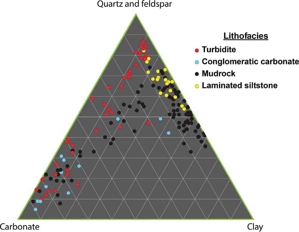
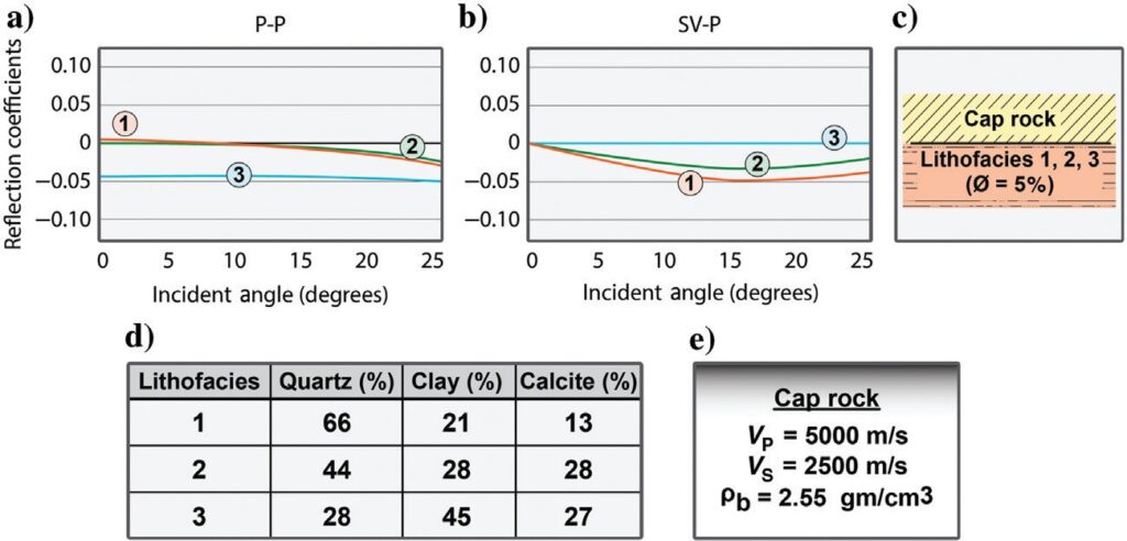
An illustration of the fundamental difference in P-P and SV-P reflectivity physics for Wolfberry turbidites is demonstrated by data displayed in Figures 8 and 9. The erratic distribution of minerals in low-porosity, low-permeability Wolfberry lithofacies is illustrated in Figure 8. These insights into the mineral fabric of Wolfberry depositional units were determined by a laborious, detailed, mineral count in thin sections cut from 182 Wolfberry cores (Hamlin and Baumgardner, 2012). Mineral mixtures observed in these thin sections are the data plotted in Figure 8. These X-ray diffraction data, coupled with the log facies in Figure 2, indicate that the mineralogical composition of Wolfberry turbidites can vary in dramatic fashion between immediately adjacent Wolfberry facies units.
This ground truth insight into the complexity of mineral mixtures that form Wolfberry rock fabric is used in the reflectivity modeling illustrated in Figure 9. Elastic coefficients of each mineral component in mineral mixtures 1, 2, 3 identified in Figure 9d were combined to construct the elastic properties of hypothetical Wolfberry facies units that form the lower layer of the two-layer model in Figure 9c. The methodology used to create composite rocks that have matrices with specific percentages of quartz, clay, and calcite was patterned after a procedure proposed by Hill (1965). The P-P and SV-P reflection behaviors in Figure 9a and 9b were then calculated for the boundary separating the two rock units shown in Figure 9c.
Reflectivity curves in Figure 9a indicate that rock boundaries 1 and 2 would be invisible, or quite weak at best, in a P-P image, but rock boundary 3 would create a robust P-P reflection. In contrast, the SV-P reflectivity curves in Figure 9b show that rock boundary 3 would not appear in an SV-P image but rock boundaries 1 and 2 would produce respectable SV-P reflections. These opposite outcomes illustrate a fundamental axiom of seismic stratigraphy that needs to be applied when analyzing Wolfberry turbidites: P-P images and SV-P images will differ in some areas of image space, yet both images can still be correct. Said another way, SV-P data provide seismic interpreters a different set of Wolfberry stratal surfaces than do P-P data, and both sets of stratal surfaces (SV-P and P-P) should be used in stratigraphic studies of the Wolfberry interval. The seismic interpretation community does not yet practice S-wave seismic stratigraphy and uses only P-P data in seismic stratigraphy studies. Perhaps with the knowledge that S-mode seismic stratigraphy can be practiced with SV-P data extracted from vertical-geophone data, attention to using P and S data in a unified seismic stratigraphy interpretation will begin to be practiced.
Extracting turbidite geobodies from SOM volumes The term geobody is often used to designate a distinct definable component of a depositional system. The size, shape, and location of a geobody extracted from seismic data will change when different criteria are used to identify seismic geobodies. In our study, unsupervised ML was used to train neurons on P-P and SV-P attribute volumes so that each neuron could search for combinations of attribute coordinates where clusters of seismic attributes provided a best match with each other in attribute space. Each winning neuron found a significant number of P-P and SV-P attribute co- ordinates that satisfied that neuron’s search parameters. Families of x-y-z coordinates that constitute a distinct seismic geobody in the seismic survey space are also found in the seismic attribute space. If there are other seismic geobodies elsewhere in the seismic image space that have a specific combination of seismic attributes, these geobodies will also be found at the same x-y-z coordinates in each attribute space. These common seismic geobodies “stack” at their consistent coordinates in the attribute space.
The power of multi-attribute ML is that the stacking of one or more seismic geobodies occurs in a common natural cluster in attribute space. For completeness, it should be stated that not all winning neurons locate geologically important seismic geobodies. Some detected geobodies are not geologic but are clumps of random noise. Others are acquisition footprints, multiples, or other coherent noise events. An interpreter has to decide which geobodies are important and which have no geologic value.
A winning neuron is associated with a natural cluster in the attribute space. Such natural clusters represent concentrations of seismic samples that possess roughly the same combination of attribute values. In essence, a winning neuron may represent more than one seismic geobody if those geobodies share the same combination of attributes discovered by ML. Winning neurons align with these natural clusters. Not all winning neurons identify geologic geobodies, but all similar seismic geobodies do align with the same center of coherent energy revealed in attribute space. Sorting out which seismic geobodies are geologic and which are not is a new domain of ML assistance in seismic interpretation that will be continually improved.
This paper discusses how readily available ML interpretation of P-P and SV-P data can take interpreters deeper into their understanding of how Wolf- berry seismic geobodies are related to Wolfberry geologic geobodies. The starting point that we invoked was to invoke the premise that Wolfberry P-P and SV-P seismic responses are based on the mineralogy properties of Wolfberry rocks (Figure 9). When, as indicated in Figure 8, mineral mixture 1 occurs in a portion of one Wolfberry turbidite, but mineral mixture 2 occurs in a portion of turbidite unit 2, then turbidite 1 and turbidite 2 have different stiffness coefficients. When the rock stiffness coefficients change between coordinates 1 and 2, the seismic attributes also vary between coordinates 1 and 2. In unsupervised ML, searching neurons will identify the area around coordinates 1 as geobody 1 and the area around coordinates 2 as geobody 2.
A geobody identified in this study is thus probably best described as a seismic object that has a different rock fabric than the rock fabric associated with other detected geobodies. This premise caused the terminology “fabric and internal architecture of turbidites” to be used in the title of this paper. A geobody identified in this study should not be assumed to be an individual turbidite but to be a rock volume inside stacked Wolfberry turbidites in which there is a reasonably consistent rock fabric.
The number of neurons that search through seismic attribute space is defined by the person doing a seismic interpretation. In this study, 64 searching neurons were used for training, and each resultant winning neuron was identified with a specific color. Just like a display of seismic data products with a color scale has been a valuable interpretation tool for several decades, SOM winning neurons are also identified with a 2D color map. The 2D eight-cell by eight-cell color maps dis- played in Figure 10 identify the colors assigned to the 64 winning neurons that searched the P-P attribute space (Figure 10a) and the colors assigned to the 64 winning neurons that searched the SV-P attribute space (Figure 10b).
The neurons shown in Figure 10 are assigned a hexagonal shape, which allows each neuron to have two to six immediate neighboring neurons. Information passes through each of the six membranes around a neuron to its immediate neighbors. If neuron A decides to move a distance X toward natural attribute cluster C, this cross-membrane information sharing causes its immediate neighbors to move a small fraction of X toward C. This process is one training step for only neuron A and its immediate neighbors. When similar decisions and movements occur for every neuron (64 neurons in this study), one training step has occurred for the total neuron population. This neuron training continues until neuron migration efforts fail to advance a neuron a specified distance. At the end of the training, each neuron has found its natural clusters of attributes.
The choice of 64 searching neurons in this study was an arbitrary decision. Other interpreters may prefer to reduce their winning-neuron map to a 5 × 5 grid and use only 25 searching neurons or to use a 10 × 10 color grid and increase the number of searching neurons to 100. Geobodies will have different sizes and shapes as the dimensions of a winning-neuron map vary, i.e., as the number of winning neurons varies. Interpreters have to decide what population of neurons best provides the information they seek.
When each searching neuron, during its training, finds a data point where there is the combination of seismic attributes that it seeks, the x-y-z coordinates of that image point are assigned to that neuron’s colored cell. At the conclusion of all neuron migrations through the multidimension attribute space, each colored cell in each 2D winning-neuron map in Figure 10 contains several tens to several thousands of sets of x-y-z coordinates that define where each winning neuron should be distributed in the seismic attribute space.
A color display of a seismic data volume that uses only one cell from a 2D SOM winning-neuron map (e.g., cell 14 in Figure 10a) defines the spatial distribution throughout the P-P x-y-z space where winning-neuron 14 found its unique combination of P-P seismic attributes during neuron training. This spatial distribution where neuron 14 was the winning neuron may be a population of only a few x-y-z coordinates, or it may be a population of several hundreds of x-y-z coordinates.
A display of these single-color seismic coordinates identifies seismic geobodies that have similar seismic attribute properties. For example, seismic samples associated with seismic geobodies identified by SOM winning-neuron index 37 will be colored a dark blue with the color map of Figure 10a. The same seismic geobodies would be colored a yellow shade if the color map of Figure 10b is used. A seismic image created by SOM classification is a valuable interpretation tool. The choice of number of winning neurons and the choice of colors assigned to those neurons are arbitrary, but important, decisions made by each seismic interpreter.
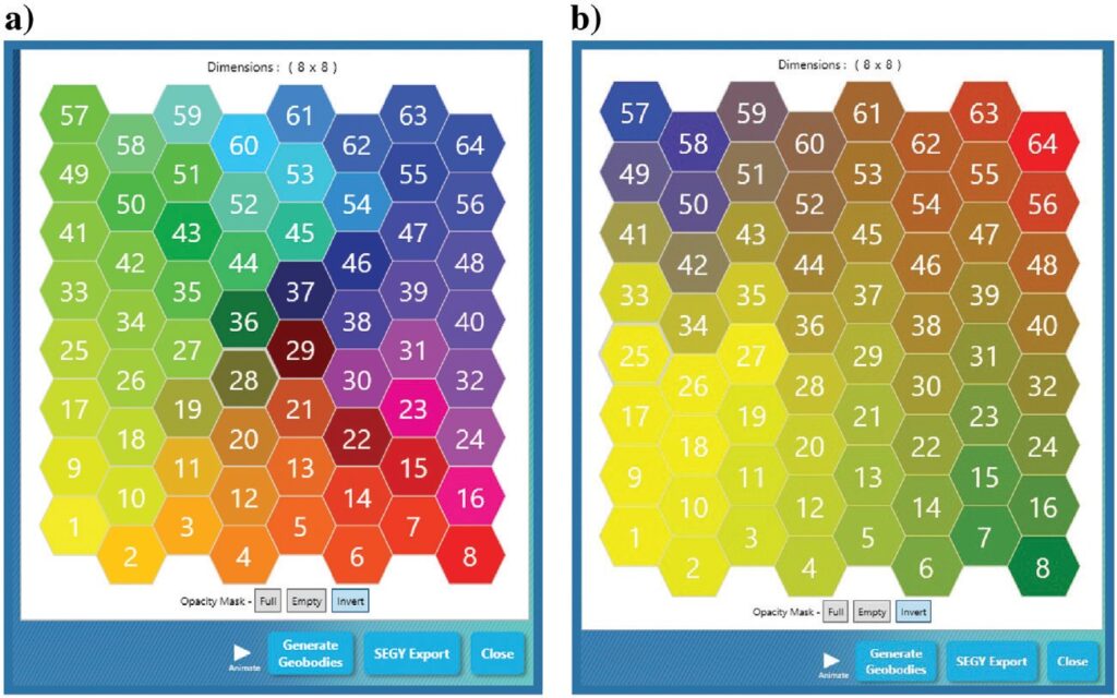
the 64 neurons that searched the SV-P attribute space. Each neuron is depicted as a hexagon with six straight sides and six internal angles of 120°. During neuron training, varying degrees of information sharing occur between neighboring neurons.
Examples of P-P Wolfberry geobodies are shown in map view in Figure 11. Figure 11a is a constant-time horizontal slice through the P-P data volume. This horizontal slice is positioned slightly more than one-fourth of the Wolfberry interval below the top of the Spray- berry, and all 64 colors of the P-P SOM in Figure 10a are active. It is difficult to interpret individual Wolfberry regions with this display format. In fact, based on just this one volume slice, it is challenging to even state that the imaged geology is a turbidite system.
When specific P-P geobodies are examined, however, there are better pictures of Wolfberry turbidite deposition. Figure 11b shows the P-P geobody associated with only color cell index 28 (i.e., winning neuron index 28) of Figure 10a. Now, there are indications of waves of turbidite deposition coming from the north- west. The arrow in the upper-left corner of the display depicts an inferred direction of sediment flow. The orientation of this depositional-flow arrow is approximately the azimuth direction from the mouth of the San Simon Channel to the study site (Figure 1). A tentative model of the internal fabric and architecture of Wolfberry turbidites at this location can begin to be constructed by assuming that each P-P winning neuron (e.g., neuron index 28) represents a unique mixture of inflowing turbidite minerals. This assumption is based on the variable mineralogy of Wolfberry turbidites exhibited in Figure 8 and on the P-P mineralogy-dependent reflectivity physics illustrated in Figure 9.
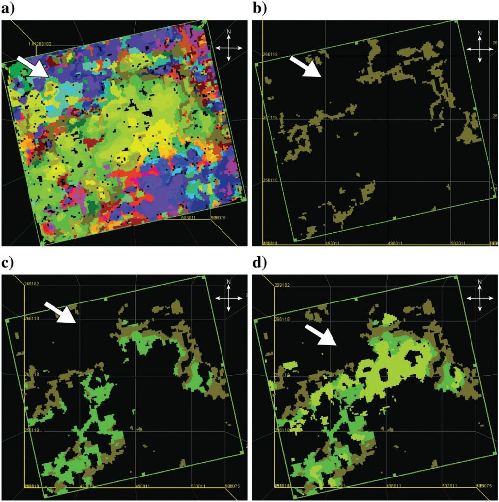
In Figure 11c, the P-P geobody associated with P-P winning neuron index 35 is added, and in Figure 11d, the geobody associated with P-P winning neuron index 26 is added. These latter displays indicate that each P-P geobody could be interpreted as a turbidite influx that transports a unique combination and percentage-mixture of matrix-forming minerals. Each P-P geobody contributes to the internal architecture and fabric of Wolfberry turbidites. This methodology takes interpreters a long way toward understanding the geologic processes that built Wolfberry turbidites and the turbidite architecture and fabric resulting from these processes.
Winning neurons 28, 35, and 26 are near neighbors in a small region of the SOM, which means that self-organization will cause their associated natural clusters to be near neighbors in an SOM result. For example, Figure 10a shows that neurons 26, 28, and 35 communicate with each other through their common connections to neuron 27. Figure 11 then shows that indeed geobodies 26, 28, and 35 nestle against each other in the multi-attribute space.
SOM analysis is expanded to SV-P geobodies using the progression of winning neurons displayed in Figure 12. Figure 12a shows a horizontal time slice positioned almost one-third of the Wolfberry interval below the top of the Sprayberry. This full-color display reveals repeated rows of seismic facies aligned approximately southwest to northeast. Figure 12b shows the SV-P geobody identified by SV-P winning neuron index 40 of Figure 10b. The SV-P geobody associated with SV-P winning neuron index 30 is added in Figure 12c, and the SV-P geobody associated with SV-P winning neuron index 25 is added in Figure 12d. Figure 10b shows that neurons 25, 30, and 40 are well separated in the SV-P SOM grid and thus do not share significant information with each other. As a result, geobodies 25, 30, and 40 in Figure 12 are separated from each other, and the separation distances between these three geobodies in Figure 12d are roughly proportional to the distance between neurons 25, 30, and 40 in their winning-neuron grid (Figure 10b).
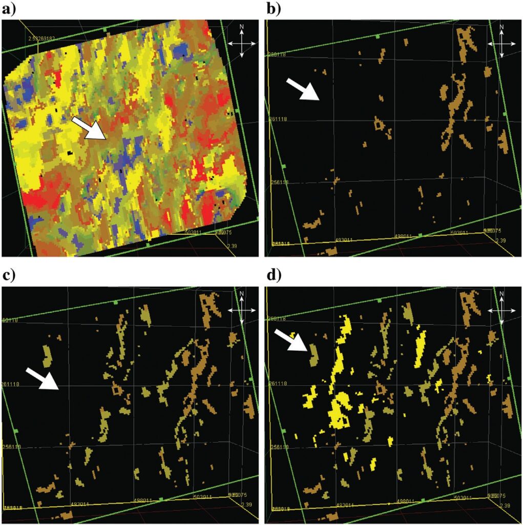
All of these SV-P geobodies have an orientation that seems to conform with a consistent sediment provenance. By repeated additions of SV-P winning neurons onto the horizontal time slice, the internal architecture and fabric of Wolfberry turbidites, as defined by SV-P reflectivity, react to different mineral mixtures of incoming sediment (Figure 9). As a result, the positions and orientations of elements in the full-color SV-P winning-neuron displayed in Figure 12a differ from the positions and orientations of elements that comprise the P-P winning-neuron display in Figure 11a.
A tentative working hypothesis is that these dual P-P and SV-P SOM geobody analyses allow interpreters to not only have a broader understanding of the internal architecture of Wolfberry turbidites but to also have a possible picture of the distributions of mineral mixtures within Wolfberry turbidites.
Conclusions
Interpreting Wolfberry seismic images with unsupervised ML software exposes details about the internal architecture and fabric of Wolfberry turbidites that cannot be seen with conventional seismic interpretation procedures. Principal component and SOM analyses are invaluable for determining which seismic attributes, used in what percentage combinations, provide maximum information about Wolfberry turbidites. It is advisable, and probably essential, that principal components used in ML interpretations of Wolfberry turbidites be calculated in seismic volumes constrained to the Wolfberry turbidite interval. Principal components created to describe Wolfberry turbidites should not be influenced by data that image nonturbidite geology.
SOMs are effective tools for visualizing how natural clusters of combinations of Wolfberry seismic attributes are distributed in attribute space. Once a SOM of Wolfberry attributes, picked with the aid of principal components, is displayed with an appropriate color palette, seismic geobodies embedded in Wolfberry geologic turbidites can be extracted and analyzed. Each geobody represents the spatial distribution of a specific weighted-combination of seismic attributes found in the Wolfberry image space by unsupervised ML in the attribute space.
This study shows that SV-P data are valuable for imaging Wolfberry turbidites. SV-P images show turbidit-like Wolfberry features with quality equal to, and sometimes better than, features observed in P-P data. Because P-P reflectivity and SV-P reflectivity react to different interfaces in a propagation medium where rocks have spatially varying mineral mixtures, SV-P data contain geobodies that describe a different set of gravity-driven mineral distributions than do geobodies extracted from P-P data.
Rock-physics analysis of the effects that alterations in mineral mixtures of a rock matrix have on P-P and SV-P reflectivity introduces the concept that Wolfberry geobodies define volumes inside stacked Wolfberry turbidites where there are unique combinations of fabric-forming minerals. P-P attributes contain geobody information that respond to the effects that mineral composition has on P-P reflectivity; similarly, SV-P attributes contain geobodies that respond to the effects that mineral composition has on SV-P reflectivity. This tentative hypothesis provides two independent descriptions of the internal architecture and fabric of Wolfberry turbidites. Future work needs to focus on how these two sets of geobodies (a P-P set of geobodies and an SV-P set of geobodies) should be integrated into a coherent description of the internal fabric and architecture of a turbidite system and the provenance of turbidite-forming sediments.
Wolfberry operators should examine their legacy P-source seismic data and determine if P-source data recorded by vertical geophones contain SV-P reflections of usable quality. The image value of SV-P data is too great to continue to ignore the fact that SV-P reflections exist in thousands of square miles of legacy P-source data and are available for imaging exploration targets at zero data-acquisition cost.
Acknowledgments
We thank Leah Mann of Advertas Inc. for preparing the graphics for this publication.
Data and materials availability
Data associated with this research are confidential and cannot be released.
References
Aki, K., and P. G. Richards, 1980, Quantitative seismology — Theory and methods: W.H. Freeman and Co.
Aki, K., and P. G. Richards, 2002, Quantitative seismology— Theory and methods: W.H. Freeman and Co.
Bishop, C. M., 2006, Pattern recognition and machine learning: Springer, 561–565.
Brito, M., 2010, Principal component analysis for stratigraphic imaging improvement and facies predictions: 80th Annual International Meeting, SEG, Expanded Abstracts, 2401–2405, doi: 10.1190/1.3513333.
Chopra, S., and K. J. Marfurt, 2014, Churning seismic attributes with principal component analysis: 84th Annual International Meeting, SEG, Expanded Abstracts, 2672–2676, doi: 10.1190/segam2014-0235.1.
Frasier, C., and D. Winterstein, 1990, Analysis of conventional and converted mode reflections at Putah Sink, California using three-component data: Geophysics, 55, 646–659, doi: 10.1190/1.1442877.
Guo, H., K. J. Marfurt, and J. Liu, 2009, Principal component spectral analysis: Geophysics, 74, no. 4, P35–P43, doi: 10.1190/1.3119264.
Gupta, M., and B. Hardage, 2017, Improved reservoir delineation by using SV-P seismic data in Wellington field, Kansas: 87th Annual International Meeting, SEG, Expanded Abstracts, 5182–5186, doi: 10.1190/segam2017-17559574.1.
Hamlin, S., and R. Baumgardner, 2012, Wolfberry (Wolfcampian-Leonardian) deep-water depositional systems in the Midland Basin — Stratigraphy, lithofacies, reservoirs, and source rocks: Report of Investigations No. 277, Bureau of Economic Geology, The University of Texas at Austin.
Hardage, B. A., 2017a, Practicing S-wave reflection seismology with “P-wave” sources — Concepts, principles, and overview: 87th Annual International Meeting, SEG, Expanded Abstracts, 5152–5156, doi: 10.1190/segam2017-17256173.1.
Hardage, B. A., 2017b, Examples of SV-P images made with P sources and vertical geophones: 87th Annual International Meeting, SEG, Expanded Abstracts, 5187– 5191, doi: 10.1190/segam2017-17430569.1.
Hardage, B. A., 2017c, Real-data comparisons of direct-S modes produced by “P” sources and “gold standard” S sources: 87th Annual International Meeting, SEG, Expanded Abstracts, 2481–2485, doi: 10.1190/segam2017-17430461.1.
Hardage, B. A., 2017d, Land based S-wave reflection seismology with P sources — Does it work?: 87th Annual International Meeting, SEG, Expanded Abstracts, 6067–6071, doi: 10.1190/segam2017-w11-04.1.
Hardage, B. A., D. Sava, and D. Wagner, 2014, SV-P — An ignored seismic mode that has great value for interpreters: Interpretation, 2, no. 2, SE17–SE27, doi: 10.1190/INT-2013-0096.1.
Hardage, B. A., and D. Wagner, 2014a, Generating direct-S modes with simple, low-cost, widely available seismic sources: Interpretation, 2, no. 2, SE1–SE16, doi: 10.1190/INT-2013-0095.1.
Hardage, B. A., and D. Wagner, 2014b, S-S imaging with vertical-force sources: Interpretation, 2, no. 2, SE29– SE38, doi: 10.1190/INT-2013-0097.1.
Hardage, B. A., and D. Wagner, 2018a, Direct-SV radiation produced by land-based P sources — Part 1: Surface sources: Interpretation, 6, no. 3, T569–T584, doi: 10.1190/INT-2018-0046.1.
Hardage, B. A., and D. Wagner, 2018b, Direct-SV radiation produced by land-based P sources — Part 2: Buried explosives: Interpretation, 6, no. 3, T585–T599, doi: 10.1190/INT-2018-0047.1.
Haykin, S., 2009, Neural networks and learning machines, 3rd ed.: Pearson.
Hill, R., 1965, A self-consistent mechanics of composite materials: Journal of the Mechanics and Physics of Solids, 13, 213–222, doi: 10.1016/0022-5096(65) 90010-4.
Karr, B., 2017, SV-P imaging compared to P-SV imaging — Analysis of statics and velocities required to create an SV-P image: 87th Annual International Meeting, SEG, Expanded Abstracts, 5177–5181, doi: 10.1190/segam2017-17728712.1.
Kohonen, T., 2001, Self organizing maps: Third extended addition: Springer, Series in Information Services.
Li, Y., and B. A. Hardage, 2015, SV-P extraction and imaging for far-offset vertical seismic profile data: Interpretation, 3, no. 3, SW27-SW35, doi: 10.1190/INT-2015-0002.1.
Li, Y., D. Wang, S. Shi, and X. Cui, 2017, Gas reservoir characterization using SV-P converted wave mode — A case study from western China: 87th Annual International Meeting, SEG, Expanded Abstracts, 5172–5776, doi: 10.1190/segam2017-17726552.1.
Roden, R., T. Smith, and D. Sacrey, 2015, Geologic pattern recognition from seismic attributes: Principal component analysis and self-organizing maps: Interpretation, 3, no. 4, SAE59–SAE83, doi: 10.1190/INT-2015-0037.1.
Wagner, D., and B. A. Hardage, 2017, Using finite-difference modeling to understand direct-SV illumination produced by P sources: 87th Annual International Meeting, SEG, Expanded Abstracts, 5167–5171, doi: 10.1190/segam2017-17661718.1.
Wilmott, P., 2019, Machine learning — An applied mathematics introduction: Panda Ohana Publishing.