Deep Learning for Characterizing Paleokarst Collapse Features in 3-D Seismic Images

Abstract

Paleokarst systems are found extensively in carbonate-prone basins worldwide. They can form large reservoirs and provide efficient pathways for hydrocarbon migration, but they can also create serious engineering geohazards. The full delineation of potentially buried paleokarst systems plays an important role for reservoir characterization, oil and gas production, and other engineering tasks. We propose a supervised convolutional neural network(CNN) to automatically and accurately characterize paleokarst and associated collapse features from 3-D seismic images. To avoid time-consuming manual labeling for training the CNN, we propose an efficient workflow to automatically generate numerous 3-Dtraining image pairs including synthetic seismic images and the corresponding label images of the collapsed paleokarst features simulated in the seismic images. With this workflow, we are able to simulate realistic and diverse geologic structures and collapsed paleokarst features in the training images from which the CNN can effectively learn to recognize the collapsed paleokarst features in real field seismic images. Two field examples from the Fort Worth Basin demonstrate that our CNN-based method is superior to conventional automatic methods in delineating paleokarst collapse features from seismic images. From the CNN-based paleokarst characterization, we can further automatically extract 3-Dcollapsed paleokarst systems and quantitatively measure their geometric parameters. Our CNN-based method is highly efficient and takes only seconds to classify collapsed paleokarst features a 3-D seismic image with 320×1, 024×1, 024 samples (approximately 268 km2) by using one graphics processing unit.

1. Introduction

Karst is a typical type of carbonate terrain that has gone through significant diagenetic processes, which often generate associated structural features of joints, caves, faults, and collapses (Qi et al., 2014). Buried, collapsed paleokarst systems can form carbonate petroleum reservoirs including those explored in the Fort Worth Basin (FWB) (e.g., Dou et al., 2011; Kerans, 1988; Loucks & Anderson, 1985), the Lower Cretaceous Golden Lane field in eastern Mexico (Coogan et al., 1972; Viniegra & Castillo-Tejero, 1970), the Tarim Basinin China (e.g., Desheng et al., 1996; Maoshan et al., 2011; Qi et al., 2014; Zeng et al., 2011), and other paleokarst-related fields reported in previous works (e.g., Andre & Doulcet, 1970; Loucks, 1999; Mazzullo & Mazzullo, 1970; Zhai & Zha, 1982). In addition, collapsed paleokarst systems pose potential drilling hazards due to the weakness of the paleokarst zones (Qi et al., 2014; Soriano et al., 2019; Zhao et al., 2018). Therefore, delineating subsurface collapsed paleokarst systems is important for petroleum reservoir characterization and production.

Three-dimensional seismic images are widely and commonly used to map paleokarst systems and to study paleokarst related features. To facilitate the paleokarst interpretation in 3-D seismic images, some seismic attributes including coherence (Bahorich & Farmer, 1995; Li & Lu, 2014; Marfurt et al., 1999), structural curvature (Al-Dossary & Marfurt, 2006; Di & Gao, 2016; Roberts, 2001), reflector rotation (Marfurt &Rich, 2010), and spectral decomposition (Chen, 2016; Qi & Castagna, 2013) are calculated to highlight the paleokarst features in 3-D seismic images. Automatic paleokarst interpretation based on such attributes alone, however, remains challenging because these attributes are typically sensitive to noise and other types of structural discontinuities or variations that are unrelated to the collapsed paleokarst features. Significant human interactions are still required to delineate the collapsed paleokarst systems by integrating multiple types of seismic attributes (Khatiwada et al., 2013; Qi et al., 2014; Sullivan et al., 2006; Zhao et al., 2018)

We propose a convolutional neural network (CNN) to fully detect paleokarst collapse features in 3-D seismic images and extract 3-D paleokarst chimney tubes all at once, which would provide a clear 3-D perspective of he collapsed paleokarst systems in the subsurface. CNN-based methods are powerful for multidimensional image processing tasks including image classification (e.g., He et al., 2016; Krizhevsky et al., 2012; Simonyan & Zisserman, 2014; Szegedy et al., 2015), object detection (e.g., Lin et al., 2017; Liu et al., 2016; Redmonet al., 2016; Ren et al., 2015; Sermanet et al., 2013), and image segmentation (e.g., Badrinarayanan et al., 2017; Chen et al., 2017; Long et al., 2015; Ronneberger et al., 2015). Recently, CNNs have been increasingly applied in geoscience problems (Bergen et al., 2019; Bianco et al., 2019) including the interpretation of geologic faults(e.g., Di et al., 2019; Lu et al., 2018; Wu, Liang, et al., 2019; Wu, Shi, et al., 2019; Zhao & Mukhopadhyay, 2018),horizons (e.g., Geng et al., 2019; Wu, Zhang, et al., 2019; Wu et al., 2020), salt bodies (e.g., Di & AlRegib, 2020; Di et al., 2018; Guillen et al., 2015; Shi et al., 2019), and channels (Pham et al., 2019) in seismic images.

In this paper, we consider the characterization of paleokarst collapse features in a 3-D seismic image as an image segmentation problem and solve this problem by using a supervised CNN. The architecture of our CNN is modified from the U-net (Ronneberger et al., 2015) by upgrading the convolutional layers from 2-D to 3-D and reducing the number of layers and features at each layer, which significantly saves GPU memory and makes it applicable to our task of processing 3-D large seismic images. Training a CNN typically requires a large amount of training data sets including input images and the corresponding label images. In our problem of collapsed paleokarst interpretation in seismic images, however, we lack the input seismic images, especially labeled images with interpreted paleokarst features. Manually interpreting or labeling the paleokarst in seismic images is time-consuming, which makes it hard to prepare a large amount of reliable or diverse label images for training a CNN.

To solve this problem of lacking training data sets, we propose a workflow to automatically generate numerous synthetic seismic images, where a variety of realistic structural patterns and collapsed paleokarst features are simulated with well-defined functions. The collapsed paleokarst features in these generated synthetic seismic images are well defined, and we are able to automatically obtain the corresponding label images with the ground-truth of collapsed paleokarst features. With this workflow, we automatically generate 100 pairs of 3-D synthetic seismic images and the corresponding labeled paleokarst images. These100 pairs, with further data augmentation, are proven sufficient to train our CNN for collapsed paleokarst characterization in 3-D seismic images. Although trained only by synthetic seismic images, our CNN shows powerful performance in delineating collapsed paleokarst features in field seismic images. The detected paleokarst results are consistent with previous manual interpretations and are superior to the collapsed paleokarst features characterized by conventional seismic attributes of curvature and coherence. From the images of collapsed paleokarst features computed by the trained CNN, we are able to automatically extract the boundaries of 3-D collapsed paleokarst systems, which may be extensively and complicatedly developed in a 3-D seismic image. Based on the extracted 3-D collapsed paleokarst systems, we can further automatically measure their geometric parameters for quantitative analysis of paleokarst development.

The structure of the paper is organized as follows: We start with discussing two 3-D field seismic surveys in the FWB, the related geological background, and observations of the collapsed paleokarst features in the seismic images. We then present a novel workflow to numerically simulate realistic folding structures and collapsed paleokarst systems in 3-D synthetic seismic images. We further discuss the architecture of the proposed CNN and train it with various synthetic data sets that are automatically generated by using the proposed numerical simulation workflow. We finally demonstrate the applicability of the trained CNN with two 3-D field seismic images and compare the results with those from both manual interpretation by previous researchers and conventional automatic methods of curvature and coherence.

2. Field Seismic Data and Geologic Background

As denoted by the blue and red blocks in Figure 1, the two time-migrated 3-D seismic data sets (Figures 2a and 3a) used in this paper were both acquired at the FWB but are located at different structural settings within the basin. The first seismic data (Figure 2a) was acquired by the Bureau of Economic Geology at the University of Texas at Austin and its industry partners including Arch Petroleum, Enserch, and Oxy USA (Hardage, 1996). As denoted by the blue block in Figure 1a, the corresponding seismic survey covers an area of 67 km2at the Boonsville field in the northern FWB. The Boonsville field (colored cyan in Figure 1a) is one of the largest gas fields in the United States. The second seismic image (Figure 3a) is from the central FWB by the Marathon Oil Company with 16 live receiver lines, forming a 324 km2wide-azimuth survey (red block in Figure 1a) with a fine 16×16 m2Common Depth Point (CDP) bin size (Qi et al., 2014).

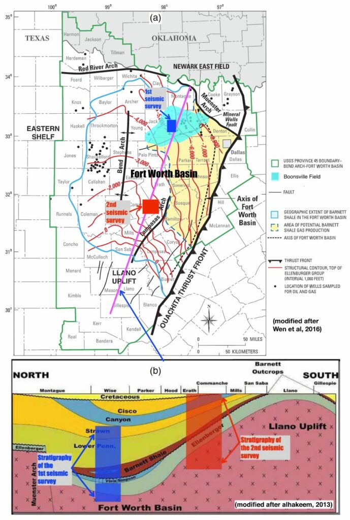
The FWB is a major petroleum producing geological system which has yielded over 120 billion of gross production since 2001 (George, 2016). The FWB is formed along the Ouachita thrust front as shown in Figure 1a. It is a wedge-shaped (Figure 1a), asymmetrical, and northward deepening (Figure 1b) depression with about 12,000 feet (3,657.6 m) of strata in its deepest northeast area near the Ouachita thrust belt and Muenster Arch (Figure 1a). Previous studies suggested that the FWB was formed during the late Paleozoic Ouachita Orogeny, which is a major tectonic event of thrust-fold deformation associated with the oblique lithospheric convergence of the North American and South American plates (Walper, 1982).

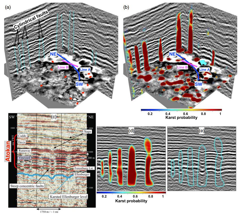
Figure 1b shows a stratigraphic cross section of the FWB from north to south as denoted by the magenta line in Figure 1a. The lower Ellenburger group of carbonate strata is unconformably overlain by the Ordovician Viola and Simpson formations, which pinch out just east of the first seismic survey (Figure 2 and denoted by the blue block in Figure 1a) (McDonnell et al., 2007) and are also missing in the second seis-mic survey (Figure 3 and denoted by the blue block in Figure 1a). Therefore, in the two study areas, the lower Ellenburger group carbonate strata are unconformably overlain by the organic-rich Barnett Formation (as shown in Figure 1b), which recorded deposition of the deep-water foreland basin during the late Mississippian (Sullivan et al., 2006) and plays a critical role in forming multiple gas fields in northern Texas (Pollastro et al., 2007). The Barnett group is overlain by the Pennsylvanian formation, which includes the Bend (lower Pennsylvanian), Strawn, and Canyon groups. As marked in Figure 2c, the Bend group (Morrowan and Atokan stages of the lower Pennsylvanian) consists of Marble Falls, Vineyard, Runawary, Davis, and Caddo stratigraphic units (McDonnell et al., 2007).

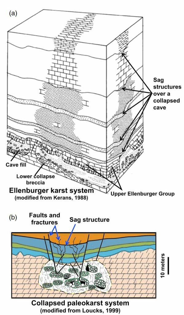
Paleokarst caves and solution collapses are extensively generated in the Ellenburger group because it went through a series of karst events ranging between the post Ellenburger and Early Pennsylvanian (Canteret al., 1993). In addition, the strata of the Silurian and Devonian strata are missing in the two study areas, which provides additional time for generating paleokarst in the Ellenburger group (Sullivan et al., 2006; Zhao et al., 2018). Figure 4a shows a model (Kerans, 1988) of the paleokarst system and the associated developments in the Ellenburger group. As shown in this model, the collapsed paleokarst system typically contains the three basic components of a paleocave floor, fill, and roof. During burial, paleocaves often collapse and sequentially produce a collapsed zone with some unique associated features as shown in the diagram (Figure 4b) of the coalesced collapsed-paleocave system proposed by Loucks (1999). According to the diagram, a coalesced collapsed paleokarst system typically contains fill deposits (breccias and stratified deposits), a broader damage zone of crackle fractures, circular faults, and chimney or sag structures (Figure 4a) in younger formations. Such collapse chimneys or sags in our seismic images vertically extend upward from the Ellenburger group through the Mississippian (e.g., Barnett Shale) and Pennsylvanian strata (as interpreted by McDonnell et al., 2007 in Figure 2c) over a distance of almost 800 m (Hardage et al., 1996).Therefore, interpreting the collapsed paleokarst-related features, especially the sags with long vertically upward extents, is important for reducing the risks of drilling and hydraulic fracturing in exploring the main oil and gas reservoirs in the Barnett Shale (deposited during the Mississippian period) and Bend group (deposited during the Middle Pennsylvanian period).

Three-dimensional seismic imaging provides an effective way to interpret the paleokarst system in the 3-D subsurface. As shown in Figures 2a and 3a, collapsed paleokarst features, especially the large-scale fault and sag structures, can be extensively observed. Manually interpreting such features, however, remains a time-consuming task, while accurately and fully delineating the paleokarst-related features in the 3-D subsurface space is challenging. We propose a CNN to efficiently and accurately segment or detect the paleokarst-collapse features from the 3-D seismic images by computing a paleokarst collapse probability volume as shown in Figures 2b, 2d, 3c, and 3d. From the probability volumes, we are able to further automatically obtain the 3-D bodies of the paleokarst chimneys or sags in the 3-D subsurface space, which provides a convenient way to quantitatively analyze collapsed paleokarst systems.

3. Seismic Simulation of Paleokarst Collapses

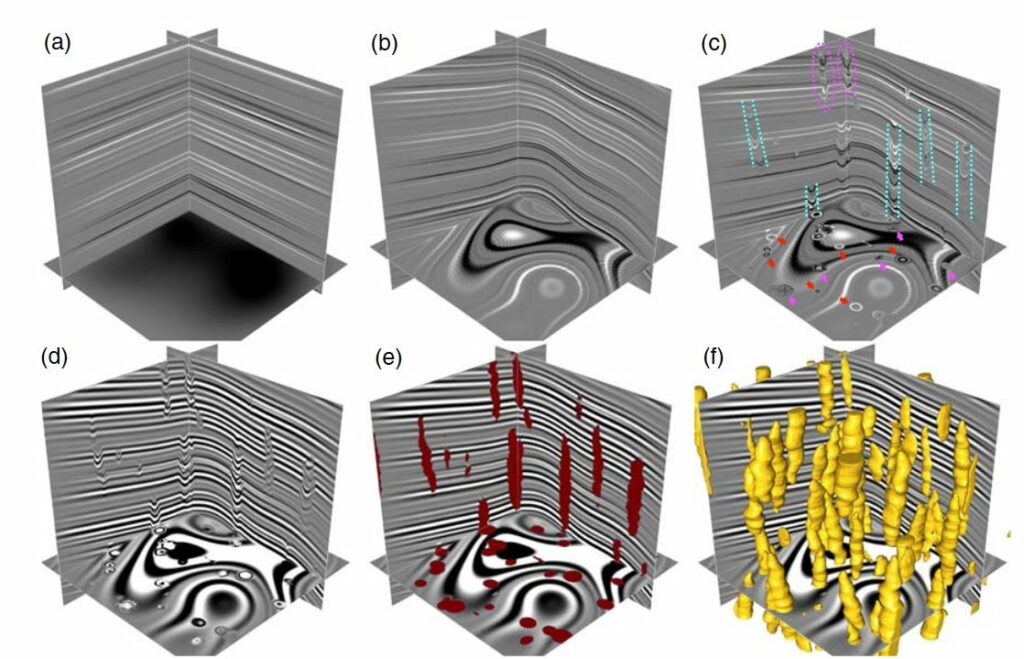
To train a CNN for segmenting the paleokarst-related features from a 3-D seismic image, we propose a workflow (as shown in Figure 5) to automatically generate many 3-D synthetic seismic images where the folding structures and collapsed paleokarst features are diverse and realistic. The well-defined collapsed paleokarst features can be automatically and perfectly labeled to obtain the target images for training the CNN.

3.1. Simulating Folding Structures

In this workflow, we begin with an initial 3-D reflectivity model r0(x,y,z) with flat layers (as shown in Figure 5a), where the reflectivity values at each layer are randomly generated and smoothly vary in space. We then randomly generate folding structures by vertically shearing the flat model, where the shearing field s(x,y,z) is defined as a combination of two functions:

where the first function s1 is a combination of N Gaussian functions scaled by a vertically damping function as suggested by Wu, Liang, et al. (2019) and Wu et al. (2020):

In defining this function, the parameters are all randomly chosen from some predefined ranges as discussed by Wu et al. (2020). By using the damping scalar function 1.5/Zmax, we gradually decrease the curvature (or bending extent) vertically upward from bottom to top in the model. The second function is simply a linear function as follows:

where the parameters p, q, and c0 are constant values that are randomly chosen for each reflectivity model. This linear function is used to generate the purely dipping structures in the reflectivity model. The slopes of the dipping structures in the x− and y− directions, respectively, are defined by the parameters p and q, which are randomly chosen from a limited range of [−0.25, 0.25] to avoid generating layers with extremely high slopes after combining with s1 (Wu et al., 2020). We set to ensure that the center trace of the reflectivity model is not shifted.

With the defined vertical shearing field we are able to compute a folded reflectivity model r(x,y,z) from the initial model r0(x,y,z) as follows:

where a classic sinc interpolation is applied to map the reflectivity model from the initially flat space to the folded or sheared space. As the parameters for defining the shearing functions are randomly chosen in generating the folded reflectivity model, the folding structures in each model are unique. In addition, each parameter has many options; therefore, we have numerous possible combinations of parameters for generating numerous folded reflectivity models with various structures.

3.2. Simulating Collapsed Paleokarst Structures

After generating the folded reflectivity model, the next step is to further simulate the collapsed paleokarst structure features in the model. Based on the observations from the field seismic images in Figures 2 and 3, the most dominant features of the collapsed paleokarst structures apparent in the seismic images are the chimneys or sags, the fractures or faults within the chimney zones, and the steep circular or cylindrical faults bounding the sags. As shown in the vertical seismic sections in Figures 2 and 3, each collapse chimney or sag is apparent as a vertically elongated tube with an approximately ellipsoidal shape. The vertically extended chimney or sag structures are cut by horizontal seismic slices, where we observe obvious circular features or onion rings (as denoted by the red and magenta arrows in Figures 2a and 3a). Such circular features indicate lateral changes in reflection time or depth due to the sag structures. Within some of the sag zones, the seismic reflections are highly chaotic or discontinuous (as denoted by the magenta arrows in Figure 3 and magenta ellipses in Figure 3b), which indicates that the deposits within these sag zones may be highly fractured or faulted.

To simulate a collapse chimney tube in the 3-D reflectivity model, we construct a 3-D vertically elongated ellipsoid

with which we define the 3-D tube area of a chimney as follows:

In the ellipsoidal function (Equation 5), p=(x,𝑦,z) represents the coordinates of a point in the 3-D reflectivity model. c=(cx,c𝑦,cz) represents the center of the ellipsoid, which is randomly chosen within the 3-D space of the model. A is a diagonal matrix defined by the three radii of the ellipsoid as follows:

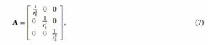
where the values of rx,ry, and rz, respectively, are randomly chosen from the predefined ranges [1, 12], [1, 12],and [4, 80] to construct ellipsoids of different sizes. Here, we set a wider range for rz to obtain primarily vertically elongated ellipsoids. In addition, we set rx>0.1rz and ry>0.1rz to avoid generating extremely longbut narrow ellipsoids that are unrealistic in practice. R is a rotation matrix that rotates the ellipsoid around the x− and y− axes as follows:

where the rotation angles 𝛼 and 𝛽 are randomly chosen from a narrow range [−10◦,10◦] to construct as lightly dipping or vertically aligned ellipsoid. By randomly choosing all the parameters in Equation 5, we are able to construct numerous possible ellipsoids with various shapes, sizes, orientations, and locations. However, in reality, a paleokarst chimney tube is not a perfect ellipsoid; we therefore randomly add some smooth perturbations to obtain irregular ellipsoids as shown in Figure 5f.

After defining the 3-D tube areas of the paleokarst chimneys, we then define the sag structures within the chimney cubes. The sag structures are typically downward bending. We therefore vertically shift the reflectors (inside a chimney cube) downward as follows to obtain a reflectivity model rk(x,y,z):

where the vertical shifts sk(x,y,z) are defined as

In this equation, f(x,y,z) is the ellipsoidal function defined in Equation 5. 𝛾 is a positive scalar that is randomly chosen from the range [10, 20]. 𝜖(x,y,z) is a random perturbation field implemented to simulate potential fractures or faults that dislocate the reflectors within the chimney tube. The perturbation field is relatively small compared to the first term of 𝛾(f(x,y,z)−1). When the perturbation field is close to 0, the shifts sk(x,y,z)≈𝛾(f(x,y,z)−1) will be nonpositive and smoothly decrease from 0 at the chimney bound to the most negative at the center of the chimney tube. In this case, the shifts will vertically shear the reflectors so that they are smoothly curved downward, as shown between the cyan dashed lines (cylindrical faults) in Figure 5c. Such generated sag structures will produce clear circular features or onion rings on the horizontal slice as denoted by the red arrows in Figure 5c. If the perturbation field is significant, the shifts sk(x,y,z) will no longer be smooth but noisy, resulting in the generation of curved and dislocated (fractured or faulted) reflectors within the chimney tubes as denoted by the magenta arrows and dashed ellipses in Figure 5c. By using this numerical method, we are able to automatically simulate various collapsed paleokarst features (as in Figure 5c) that look realistic and are comparable to the real collapsed paleokarst features in the field seismic images (Figures 2 and 3).

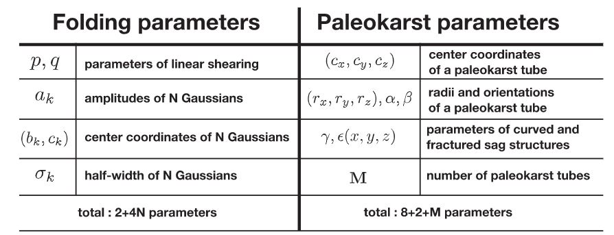
In summary, we have proposed a general workflow (Figure 5) to numerically simulate realistic folding and collapsed paleokarst structure features in a reflectivity model. The parameters used to model the folding and collapsed paleokarst features are summarized in Figure 6. A specific set of such parameters yields a reflectivity model with unique folding and collapsed paleokarst features. These parameters are not fixed but are randomly chosen to form numerous possible combinations, which allows us to generate numerous reflectivity models with various structural and collapsed paleokarst features. This is critical for our next step of training a CNN for collapsed paleokarst characterization which requires rich training data sets.

3.3. Training Data Sets

After constructing a reflectivity model (Figure 5c) with simulated folding structures and collapsed paleokarst features, our next step is to simulate a synthetic seismic image (Figure 5d) by convolving a Ricker wavelet with the reflectivity model. Instead of convolving in the vertical direction as in conventional methods, we compute the convolution here in the direction perpendicular to the reflector structures as suggested by Wu, Liang, et al. (2019) and Wu et al. (2020). The peak frequency of the Ricker wavelet is also randomly chosen from a predefined range (10–35 Hz) to compute a synthetic seismic image with various frequency components. As field seismic images are typically not as clean as the synthetic seismic image in Figure 5d, we further add random noise or the noise from field images to make the synthetic one more realistic. Figure 5eshows the corresponding label image that is automatically computed by labeling the paleokarst chimney cubes with ones while the nonkarst areas with zeros. From the label image, we can further automatically obtain the 3-D bodies of the paleokarst chimney cubes (Figure 5f) by simply calculating the isosurfaces (with isovalue 0.5) of the label image using the method of marching cubes (Lorensen & Cline, 1987).

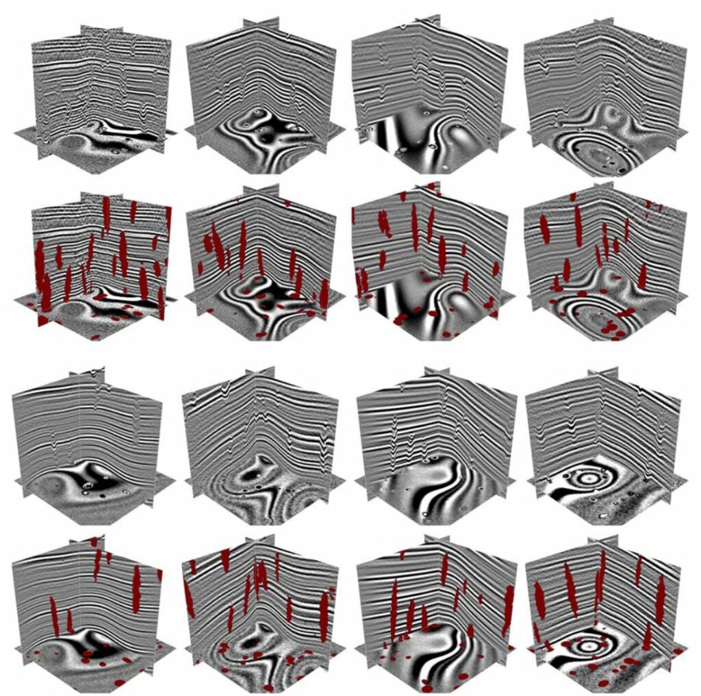
In training a CNN for detecting the collapsed paleokarst features, we need to prepare many training dataset pairs consisting of input seismic images (like the one in Figure 5d) and the corresponding label images (like the one in Figure 5e). Fortunately, in our workflow, the parameters for simulating the synthetic seismic images and the collapsed paleokarst features are not fixed. By randomly choosing the parameters, we are able to obtain numerous combinations of the parameters to calculate numerous pairs of training image with various and diverse structures and collapsed paleokarst features. In this work, we generate 120 pairs of synthetic seismic and label images, 100 pairs for training and the rest for validation. Figure 7 shows eight pairs of the automatically generated training data sets, where the first and third rows show the input seismic images, while the second and fourth rows show the corresponding label images of collapsed paleokarst features overlain with the seismic images. Notice that noise has been added to the synthetic seismic images. The noise in the first row of images is extracted from various areas of the field seismic images. The noise in the third row of images is randomly generated. In adding the noise, the noise-to-signal-ratio is randomly selected from the range [0, 0.6]. The collapsed paleokarst zones are randomly scattered in the synthetic seismic image, some are cut at the image boundaries. This is consistent with the prediction for a large field seismic image, where we often need to cut a large volume into small subvolumes and make the prediction for each subvolume.

To further increase the diversity of the training and validation data sets, we apply two types of simple data augmentation to the original 100 pairs of training data sets. The first type of data augmentation involves rotating the images around the vertical axis by 0◦,90◦, 180◦, and 270◦, which increases the number of training data sets by a factor of 4. The second type of data augmentation involves randomly cutting smaller subimages from the original images and use the subimages to train the CNN. The dimension size of each of the originally generated images is 256×256×256 (samples). During the training process, we randomly cut 128×128×128 subimages from the larger images, which ensures that the training data sets are mostly different for different training epochs. By doing this, we are able to significantly increase the number and diversity of the training data sets. In addition, training the CNN with smaller images can greatly reduce GPU memory and computational costs during the training.

4. Deep learning for Detecting Collapsed Paleokarst Features

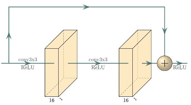
We design a CNN, as shown in Figure 8, to detect the collapsed paleokarst features in a 3-D seismic image. The architecture of the designed CNN consists of a U-shaped network followed by a residual block (Figure 9). The architecture of the 3-D U-shaped network is modified from the original 2-D U-net proposed by Ronneberger et al. (2015) for 2-D medical image segmentation, making it applicable to our 3-D problem. Compared to the original U-net, we reduce the number of layers and features at each layer to significantly save memory and computational costs which is especially important for our 3-D seismic image segmentation problem. In addition, we reduce the number of downsamplings or poolings from four to three because the dimension size (128×128×128) of our 3-D training images is relatively small and the downsampled images after four poolings would be too small (only 8×8×8) to effectively preserve the spatial or structural features in the original images.

Similar to the original U-net (Ronneberger et al., 2015), the modified U-shaped network still preserves the general architecture of a bottleneck at the middle and symmetric left contracting and right expansive paths, each of which contains three steps (reduced from four steps in the original U-net). In the left contracting path, each step consists of two 3×3×3 convolutional layers (each followed by a ReLU activation function), and a 2×2×2 max-pooling layer with stride 2. In each convolutional layer, multiple 3×3×3 filters are applied to convolve with the input image to obtain multiple output feature maps. The ReLU activation function is a nonlinear function (𝑓(x)=max(0,x)) applied to the feature maps to increase the nonlinearity of the network (Krizhevsky et al., 2012). The max-pooling layer reduces the size of the feature map by a factor of 2 and keeps only the maximum value with a 2×2×2 sliding window. At the first, second, and third steps, the numbers of feature maps at the conventional layers are 16, 32, and 64, respectively, which are significantly reduced with respect to those of the original U-net. The bottleneck at the middle contains two 3×3×3 convolutional layers, each of which contains 512 features and is, again, followed by a ReLU activation function.

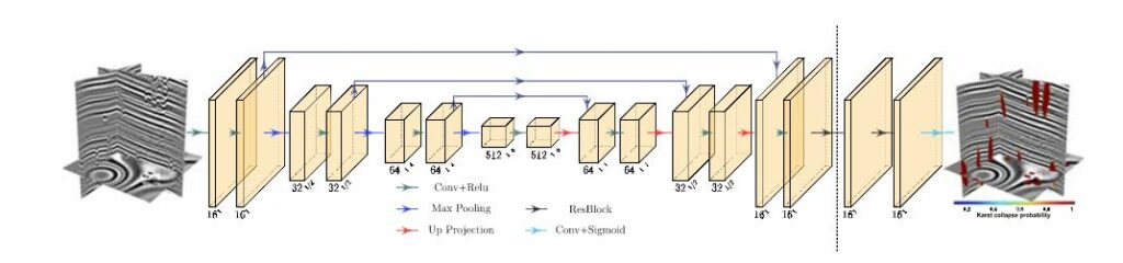
The three steps in the right expanding path gradually upsample the downsampled features back to the original size. Each step consists of a 2×2×2 upsampling operation with stride 2, a concatenation to combine the features from the left path, and two 3×3×3 convolutional layers. Each convolutional layer is followedby a ReLU activation function. The upsampling operation is implemented by using the UpSampling3D layer defined in Keras (Chollet, 2015), which increases the size of an input image by a factor of 2. After the U-shaped network, we further add another two residual blocks whose architecture is shown in Figure 9. Each residual block contains two 3×3×3 convolutional layers, each of which contains 16 features and is followed by a ReLU activation function. The final output layer is a 1×1×1 convolutional layer followed by a sigmoid activation function that generates a 3-D probability image with values in the range [0, 1] as shown on the right of Figure 8.

In constructing the network (Figure 8), the parameters of each layer are randomly initialized, which are required to be further updated to create a good mapping of an input seismic image (left of the network) toa n output paleokarst image (right of the network). Updating the network parameters involves a training process that uses an optimization algorithm to iteratively update the parameters until the error between the outputs and the label images converges on the training data set. As we consider the detection of collapsed paleokarst features a binary image segmentation problem, we use the following loss of binary cross-entropy to measure the error between the outputs and the label images:

where N is the number of samples in a 3-D output or label image and yi and pi, respectively, represent the binary label and predicted values at the ith image sample. In the training process of optimizing the network parameters, we use the Adam method (Kingma & Ba, 2014) with a learning rate of 0.0001. We iteratively train the network with 25 epochs. One epoch involves passing the entire training data set (400 pairs, including the original and rotated images) forward and backward through the neural network once. At each epoch, the training images with a smaller size 128×128×128 are cut from larger generated images (256×256×256 as in Figure 7) at random locations. Therefore, the training images at different epochs are mostly different.

In addition, each seismic image is subtracted by its mean and then divided by its standard deviation to obtain a normalized image. This normalization process is applied to ensure the amplitudes of all the seismic images are consistently distributed. Such normalizations modify the seismic amplitudes but do not change the geo-metric features or structural patterns (relative amplitude variations), from which the collapsed paleokarst features are distinguished from the nonkarst features. At each epoch of the training process, we evaluate the updated network by computing the losses and the accuracies over both the synthetic training and validation data sets. The accuracy 𝛼 is defined as follows:

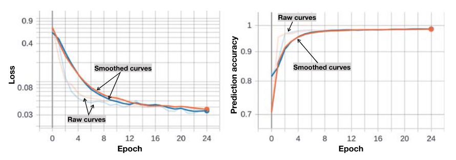
where, again, N is the number of samples in a 3-D output or label image and yi represents the binary label value at the ith image sample. ⌊pi⌉ represents the nearest integer to the predicted value pi(0≤pi≤1). We stop the training at the 25 epoch as both the training and validation losses converge to nearly 0.33, while the prediction accuracies over both the training and validation data set increase to nearly 0.99 (Figure 10).

5. Applications

To verify the effectiveness and generalization of the CNN trained with 25 epochs over the synthetic datasets, we apply the trained CNN to both synthetic and field 3-D seismic images. Although the CNN is trained by images of size 128×128×128, the size of the image input into the CNN for prediction is not fixed. This means that the trained CNN can be flexibly applied to images of arbitrary dimension sizes, so long as eachof the dimensions can be divided by 8 due to the three downsamplings included in the CNN architecture (Figure 8).

5.1. Synthetic Examples

Figure 11 shows the application of the coherence-based, curvature-based, and our CNN-based methods to four synthetic seismic images (first column in Figure 11) for collapsed paleokarst characterization. These four images (each with 256×256×256 samples) were generated by using the proposed numerical workflow (Figure 5) and are different from the images in the training data set. The first two images contain noise that is extracted from the field seismic images (Figures 2a and 3a). The second two images contain heavier random noise. The second row of Figure 11 shows the paleokarst probability images pc(x) computed from seismic coherence (Marfurt et al., 1999) as follows:

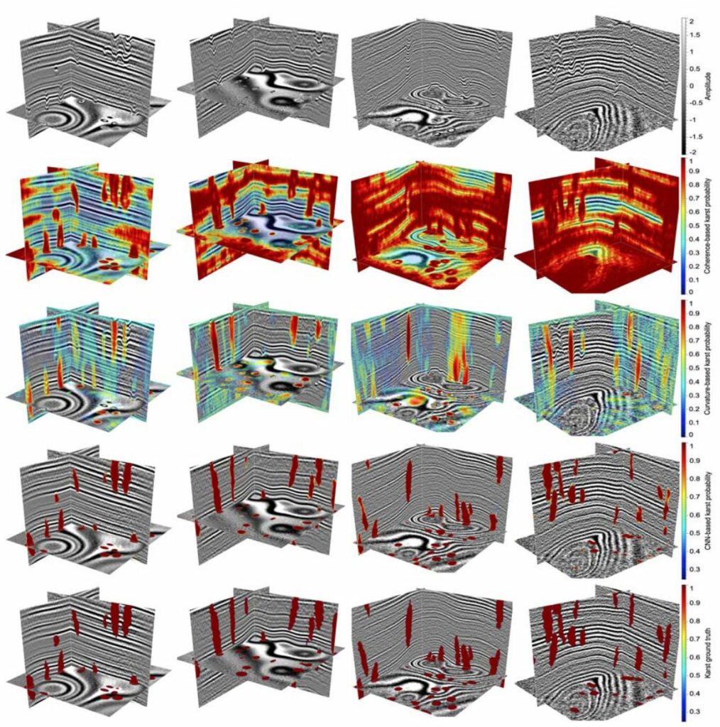
where c(x) represents a seismic coherence map that typically highlights seismic discontinuities with relatively lower values. The value of the exponent, 6, is somewhat arbitrarily chosen and is used to increase the contrast between image samples with low and high coherences. The coherence-based paleokarst probability images (second row in Figure 11) highlight most seismic discontinuities, including those in the collapsed paleokarst zones and noise.

The third row of Figure 11 shows the paleokarst probability images computed from the most positive seismic curvature Al-Dossary and Marfurt (2006) as follows:

In this equation, 𝜅(x) represents the most positive curvature map computed from an input seismic image. The structures within paleokarst collapse zones are typically curved downward and accordingly show negative values in the curvature map 𝜅(x); we therefore clip 𝜅(x) to obtain𝜅c(x) with only negative values. We further define the curvature-based paleokarst probability by using the normalized and clipped curvature map 𝜅c(x) as shown in the above equation, where the power 6, again, increases the contrast between image samples with low and high curvatures. The curvature-based paleokarst probability images (third row of Figure 11) highlight some of the collapsed paleokarst zones as well as some downward folding structures that are unrelated to the paleokarst collapses.

The fourth row of Figure 11 shows that our CNN-based paleokarst probability images visually display much more accurate collapsed paleokarst characterizations than the coherence-based and curvature-based prob-ability images. The collapsed paleokarst features highlighted (colored by red) in our CNN-based probability images are consistent with collapsed paleokarst ground truth in the label images (last row of Figure 11). In addition, our CNN-based method is highly efficient. It took only milliseconds to compute such a probability image from an input seismic image with 256×256×256 samples by using a Quadro P6000 GPU.

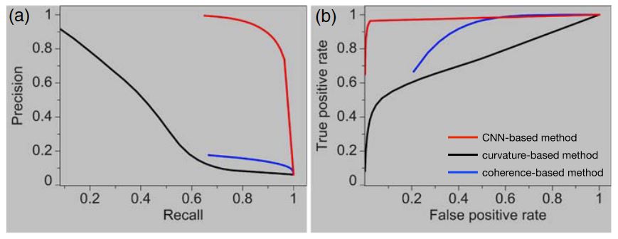
In order to quantitatively evaluate the collapsed paleokarst characterization results, we further compute precision-recall (Martin et al., 2004) and receiver operating characteristic (ROC) (Provost et al., 1998) curves as shown in Figure 12. From the precision-recall curves (Figure 12a), we observe that our CNN-based method shows the highest precision for all choices of recall. From the ROC curve, our CNN-based method shows the highest true positive rates but the lowest false positive rates.

5.2. Field Examples in the FWB

In addition to the synthetic examples in Figure 11, we further use two field examples acquired from the FWB (Figure 1a), to verify the generalization of the trained CNN to field seismic images. Compared to those in the synthetic seismic images (Figure 11), the structures and features in the field images may be significantly different.

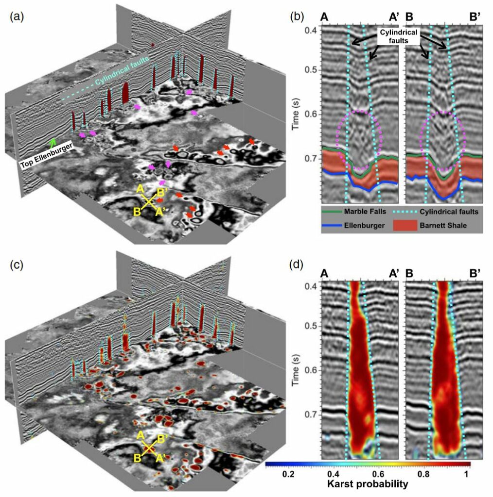
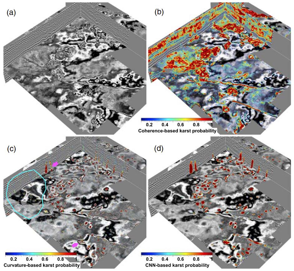
Figure 13a shows the first 3-D seismic image (the same one in Figure 3a), which was acquired at the sur-vey denoted by the red block in the FWB (Figure 1a). In this example, the paleokarst probability image (Figure 13b) computed by using the coherence-based method (Equation 13) highlights some collapsed paleokarst zones but is highly sensitive to noise. The curvature-based method (Equation 14) yields a better paleokarst probability image that detects more collapsed paleokarst zones but still contains some noisy features (e.g., the area denoted by the cyan circle) and fails to completely delineate some true paleokarst chimneys (as denoted by the magenta arrows in Figure 13c). Compared with the coherence-based and curvature-based methods, our CNN-based method yields the best probability image (Figures 3c and 13d), where the highlighted collapsed paleokarst zones are most consistent with the manual interpretation in Figure 3a.

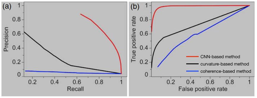
As shown in the vertical sections in Figure 3c, the boundaries of the highlighted paleokarst chimneys are consistent with the manually interpreted cylindrical faults (cyan dashed lines) bounding the chimney tubes. In Figure 3d, we display two seismic Sections AA′ and BB′ that vertically slice a large paleokarst chimney tube, where we are able to more clearly view the details of the result. In these two sections, we observe that the highlighted chimney tube starts appearing in the Ellenburger group (below the blue horizon) and continuously extends upward into the Pennsylvanian strata at the top, which is consistent with the conclusions of previous studies (e.g., Hardage et al., 1996; McDonnell et al., 2007) on the collapsed paleokarst systems in the FWB. In addition, the boundaries of the detected paleokarst chimney are highly consistent with the manually interpreted bounding cylindrical faults as denoted by the cyan dashed lines in Figures 3b and 3d. The precision-recall and ROC curves in Figure 14 show quantitative evaluations of the CNN-based (red), curvature-based (black), and coherence-based (blue) paleokarst detections compared to the manual interpretation in the two vertical sections in Figure 3a. Our CNN-based method achieves the best performance while the coherence-based method shows the worst performance on this field example.

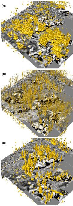
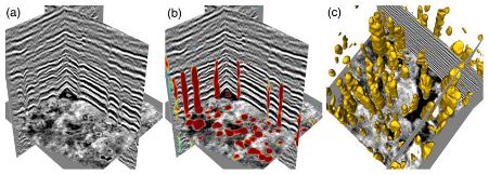
From the paleokarst probability image (Figures 3c and 13b), we can further extract the 3-D paleokarst chimney tubes (Figure 15a) by simply extracting the isosurfaces (with an isovalue of 0.5) using the method of marching cubes (Lorensen & Cline, 1987). As comparisons, Figures 15a and 15b, respectively, display the chimney tubes extracted from the coherence-based (Figure 13b) and curvature-based (Figure 13c) probability images. We observe that the tubes extracted from the coherence-based and curvature-based images contains many noisy and irregular blocks, most of which are not true paleokarst chimney tubes. In addition, the shapes of the extracted tubes are highly noisy as well, which makes it difficult to quantitatively analyze their geometries. In contrast, the 3-D chimney tubes extracted from our paleokarst probability images are geologically more reasonable and the boundaries of the tubes are more clearly presented. Most of these extracted chimney tubes narrow upward, which is consistent with the observations by McDonnell et al. (2007). From each of these extracted chimney tubes, we can automatically and accurately measure the3-D geometric parameters (e.g., diameter and vertical length) of each tube and analyze the 3-D distribution of the collapsed paleokarst systems.

The second field seismic image shown in Figures 16a and 2a is from the survey denoted by the blue block in the FWB (Figure 1)a. The collapsed paleokarst systems in this seismic image have been extensively analyzed and well interpreted by previous studies (e.g., Alhakeem, 2013; Hardage et al., 1996; McDonnell et al., 2007). In this work, we compare our automatically interpreted results using the deep learning method with collapsed paleokarst systems that are manually interpreted by McDonnell et al. (2007). Figures 2b and 16b show the automatically estimated paleokarst probability images obtained by using the our CNN. We observe that the major paleokarst chimneys are clearly highlighted in red, which correspond to relatively high probabilities.

To closely visualize the details of the detected collapsed paleokarst features and compare them with the manual interpretation results, we extract two seismic sections marked by Line A and Line B in Figures 2a and 2b. As shown in Figure 2b, Line A passes through five circular anomalies with high paleokarst probability. The extracted seismic section at Line A is shown in Figure 2c, where the paleokarst chimneys (sags)and the steep concentric or cylindrical faults were manually interpreted by McDonnell et al. (2007). Based on the manual interpretation, the paleokarst chimneys originate within the Ellenburger Group (the top of Ellenburger is marked by the blue line in Figure 2c) and extends vertically upward through the lower Atokanto the Caddo Pool Formation (McDonnell et al., 2007). Figure 2d shows the corresponding paleokarst probability section (overlain on the seismic section of Line A), where the areas of the five paleokarst chimneys are clearly highlighted. The contours (cyan curves), extracted from the probability image at the probability value of 0.5, delineate the boundaries of the paleokarst chimneys, which are consistent with the manually interpreted concentric faults (dashed black lines in Figure 2c) that bound the chimneys. Line B passes one circular anomaly with high paleokarst probabilities as shown in Figure 2b. Figure 17 shows the seismic section of Line B with manual and our automatic interpretation of the paleokarst chimney in the middle. Again, our automatic interpretation of the paleokarst chimney (Figures 17b and 17c) in this seismic section is consistent with the manual interpretation (Figure 17a) by McDonnell et al. (2007).

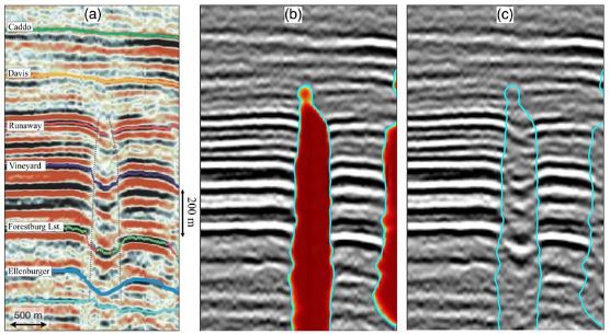
Figure 18a shows a horizontal coherency slice of the 3-D seismic image, where the chimney structures are indicated as relatively small coherence anomalies (colored in dark gray). On this coherence slice, 10 circular chimney structures are manually marked as white circles according to McDonnell et al. (2007). Figure 18b shows the corresponding horizontal slice of the paleokarst probability map overlain with the coherence slice. The circular red areas in Figure 18b denote all the automatically detected chimney structures including the 10 manually interpreted chimneys in Figure 18a. Of course, some of these detected paleokarst chimneys still need to be verified although most of them look reasonable as shown in the vertical sections in Figures 16b and 16c. By extracting the contours (with a probability value 0.5) from the paleokarst probability slice, we are able to automatically obtain the boundaries (cyan curves in Figure 18b) of all the chimneys, which provide a convenient way to quantitatively analyze the geometry of each chimney, including its shape and size.

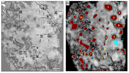
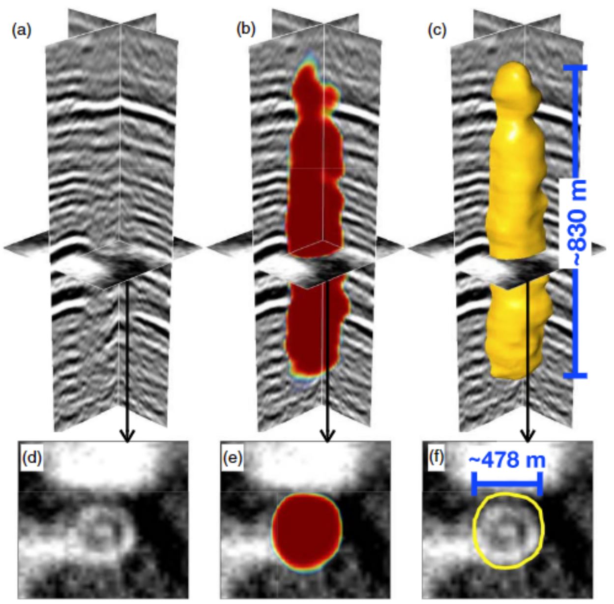
Figure 19 shows a subvolume containing the third paleokarst chimney denoted by the cyan arrows in Figures 18b and 2b. From the subvolume of the paleokarst probability map (Figure 19b), we can automatically extract the paleokarst chimney structure as a vertically extended 3-D tube, as shown in Figure 19c. Figures 19d–19f, respectively, show horizontal slices of the seismic amplitude, paleokarst probability, and extracted chimney tube. From the extracted 3-D chimney tube, we can automatically estimate the geometric parameters of the paleokarst system such as the length and width as marked in Figures 19c and 19f, which are consistent with the manual measurements provided by McDonnell et al. (2007).

6. Conclusions

We have proposed a CNN-based method to automatically delineate collapsed paleokarst features in 3-D seismic images, where the paleokarst detection is considered a problem of 3-D binary image segmentation. The architecture of the CNN is modified from the U-net, which was originally proposed for 2-D medical image segmentation and is today the most widely used network for common image segmentation problems. Specifically, we upgraded the original 2-D convolutional layers into 3-D layers and reduced the number of layers and features at each layer to make it applicable to our problem of collapsed paleokarst interpretation in 3-D seismic images.

The main challenge or limitation of applying supervised CNNs to geoscience problems, including our collapsed paleokarst interpretation, is the lack of training data sets, especially the label images or interpretation results. To solve this problem, we proposed an efficient and effective workflow to automatically generate reflectivity models with realistic folding structures and collapsed paleokarst features and then simulated the corresponding synthetic seismic images by convolving the reflectivity models with Ricker wavelets and adding some extent of random noise or real noise from field seismic images. As the folding structures and collapsed paleokarst features are well defined by functions in generating the reflectivity models, we were able to automatically obtain the corresponding label images with ground-truth collapsed paleokarst features. In addition, the parameters of functions are not fixed but randomly chosen, which makes it possible to generate numerous synthetic training data sets with various folding and collapsed paleokarst features.

Although trained with only synthetic data sets, the CNN can be applied to characterize the collapsed paleokarst features in field seismic images that are not included in the training data sets. The application of two field examples demonstrated that the collapsed paleokarst interpretation of our CNN-based methods is consistent with manual interpretations and is significantly superior to conventional automatic methods. From the CNN-based collapsed paleokarst interpretation results, we were able to automatically extract the3-D boundary of each paleokarst chimney tube in the seismic images, which enabled us to automatically measure the geometric parameters of the paleokarst tubes for quantitative analysis of the paleokarst system development.

The features of collapsed paleokarsts formed in different areas can be highly variable. However, the current trained CNN model may be limited to characterizing collapsed paleokarst systems in 3-D seismic images as we mainly simulated the collapsed paleokarst features in our synthetic training data sets. Fortunately, the current CNN model can be easily extended to delineate any type of paleokarst system by simply including more training data sets that contain the corresponding paleokarst features.

Data Availability Statement

These two seismic images are available through Hardage et al. (1996) and Qi et al. (2014). The 120 pairs of synthetic data sets, used for training and validating our CNN, are uploaded to Zenodo and are freely available through the DOI link (https://doi.org/10.5281/zenodo.3690252). The codes related to this work is available through GitHub (https://github.com/xinwucwp/KarstSeg3D) or Zenodo (https://zenodo.org/record/4013145).