There are a multitude of seismic attributes in the interpretation world today. A large group of these are referred to as single trace attributes as the computation involved in computing that attribute involves only one trace. The bulk of these attributes are based off of 5 basic attributes developed by M.Turhan Tanner, Sven Treitel, and Bob Sheriff that are referred to has the complex signal attributes or Hilbert transform attributes. These five attributes are:
- Amplitude or Real Trace
- Hilbert or Imaginary Trace
- Envelope
- Instantaneous Phase
- Instantaneous Frequency
This article will go through these 5 attributes in an overview setting and specific information can be found in the trace specific documentation included with this series.
For this explanation, a single, final stack trace will be used to illustrate these traces. This same trace will be used in all the individual attribute documentation. This comes from the Stratton field survey which is a publicly available 3D survey and is extracted from line 79, trace 89 which ties to Well # 9 which contains a VSP and full series of logs. This is a subset of the trace from 1.2 seconds to 1.6 seconds and includes two tops, C3 and F1 for reference.
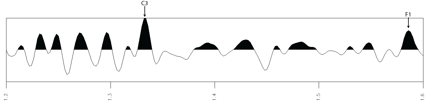 This is the amplitude or real trace.
The complex trace consists of two parts mathematically, the real (or amplitude) part and the imaginary (or Hilbert trace) part. The complex time signal c(t) combines real amplitude signal a(t) and its Hilbert transform noted as iH(a(t)) but usually shortened to H(t).
![]()
In multi-dimensional space, the real trace is shown in a vertical display with the imaginary trace perpendicular to it at the zero axis in a horizontal display. With this understanding the complex signal is a vector with one axis pointing in the real direction and the other axis pointing in the imaginary or Hilbert transform direction. The amplitude and Hilbert transform are Cartesian coordinates, X and Y, of the vector respectively. This vector can also be expressed in polar form with a vector length and angle with respect to the amplitude (X) axis.
At any instant of time the length of the vector is the Euclidean distance as indicated by the double brackets:
![]()
We call e(t) the envelope signal.
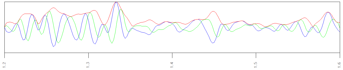
Shown are the real trace (blue), imaginary trace (green) and the envelope trace (red).
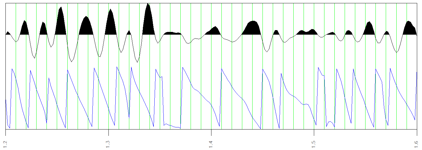
From these attributes, we can calculate out two basic measurements – the instantaneous Phase and instantaneous Frequency. Instantaneous refers to the fact that these are sample by sample calculations made down the traces, a single trace at a time.
The phase signal ![]() in Cartesian coordinate form is defined as
in Cartesian coordinate form is defined as
![]()
The phase signal ![]() in polar form is defined as
in polar form is defined as
![]()
The phase signal ![]() changes with time so we estimate the instantaneous frequency as the change of phase with time. This is the first derivative of phase over time. There are many ways to calculate derivatives, but the one often used is the following.
changes with time so we estimate the instantaneous frequency as the change of phase with time. This is the first derivative of phase over time. There are many ways to calculate derivatives, but the one often used is the following.
![]()
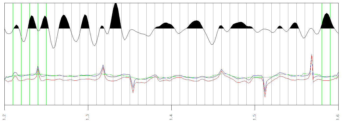
where square brackets indicate square of Euclidean distance. This is the instantaneous frequency attribute.
Here is a display of frequency ![]() in blue, smoothed frequency
in blue, smoothed frequency ![]() in green and thin bed
in green and thin bed ![]() in red. All three are included here as the thin bed is the difference between the frequency and the smoothed frequency and it makes sense to show all three.
in red. All three are included here as the thin bed is the difference between the frequency and the smoothed frequency and it makes sense to show all three.
Note that these five attributes form the foundation for most of the rest of the single trace attributes.
References:
- Taner, M. T., 2001, Seismic attributes: Canadian Society of Exploration Geophysicists Recorder, 26, no 7.