By Tao Zhao | Published with permission: SEG International Exposition and 88th Annual Meeting | October 2018
Table of contents
Summary
Within the last a couple of years, deep learning techniques, represented by convolutional neural networks (CNNs), have been applied to fault detection problems on seismic data with an impressive outcome. As is true for all supervised learning techniques, the performance of a CNN fault detector highly depends on the training data, and post-classification regularization may greatly improve the result. Sometimes, a pure CNN-based fault detector that works perfectly on synthetic data may not perform well on field data. In this study, we investigate a fault detection workflow using both CNN and directional smoothing/sharpening. Applying both on a realistic synthetic fault model based on the SEAM (SEG Advanced Modeling) model and also field data from the Great South Basin, offshore New Zealand, we demonstrate that the proposed fault detection workflow can perform well on challenging synthetic and field data.
Introduction
Benefited from its high flexibility in network architecture, convolutional neural networks (CNNs) are a supervised learning technique that can be designed to solve many challenging problems in exploration geophysics. Among these problems, detection of particular seismic facies of interest might be the most straightforward application of CNNs. The first published study applying CNN on seismic data might be Waldeland and Solberg (2017), in which the authors used a CNN model to classify salt versus non-salt features in a seismic volume. At about the same time as Waldeland and Solberg (2017), Araya-Polo et al. (2017) and Huang et al. (2017) reported success in fault detection using CNN models.
From a computer vision perspective, in seismic data, faults are a special group of edges. CNN has been applied to more general edge detection problems with great success (El- Sayed et al., 2013; Xie and Tu, 2015). However, faults in seismic data are fundamentally different from edges in images used in computer vision domain. The regions separated by edges in a traditional computer vision image are relatively homogeneous, whereas in seismic data such regions are defined by patterns of reflectors. Moreover, not all edges in seismic data are faults. In practice, although providing excellent fault images, traditional edge detection attributes such as coherence (Marfurt et al., 1999) are also sensitive to stratigraphic edges such as unconformities, channel banks, and karst collapses. Wu and Hale (2016) proposed a brilliant workflow for automatically extracting fault surfaces, in which a crucial step is computing the fault likelihood. CNN-based fault detection methods can be used as an alternative approach to generate such fault likelihood volumes, and the fault strike and dip can be then computed from the fault likelihood.
One drawback of supervised machine learning-based fault detection is its brute-force nature, meaning that instead of detecting faults following geological/geophysical principles, the detection purely depends on the training data. In reality, we will never have training data that covers all possible appearances of faults in seismic data, nor are our data noise- free. Therefore, although the raw output from the CNN classifier may adequately represent faults in synthetic data of simple structure and low noise, some post-processing steps are needed for the result to be useful on field data. Based on the traditional coherence attribute, Qi et al. (2017) introduced an image processing-based workflow to skeletonize faults. In this study, we regularize the raw output from a CNN fault detector with an image processing workflow built on Qi et al. (2017) to improve the fault images.
We use both a realistic synthetic data and field data to investigate the effectiveness of the proposed workflow. The synthetic data should ideally be a good approximation of field data and provide full control on the parameter set. We build our synthetic data based on the SEAM model (Fehler and Larner, 2008) by taking sub-volumes from the impedance model and inserting faults. After verifying the performance on the synthetic data, we then move on to field data acquired from the Great South Basin, offshore New Zealand, where extensive amount of faulting occurs. Results on both synthetic and field data show great potential of the proposed fault detection workflow which provides very clean fault images.
Proposed Workflow
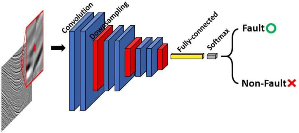
The proposed workflow starts with a CNN classifier which is used to produce a raw image of faults. In this study, we adopt a 3D patch-based CNN model that classifies each seismic sample using samples within a 3D window. An example of the CNN architecture used in this study is provided in Figure 1. Basic patch-based CNN model consists of several convolutional layers, pooling (downsampling) layers, and fully-connected layers. Given a 3D patch of seismic amplitudes, a CNN model first automatically extracts several high-level abstractions of the image (similar to seismic attributes) using the convolutional and pooling layers, then classifies the extracted attributes using the fully- connected layers, which behave similar to a traditional multilayer perceptron network. The output from the network is then a single value representing the facies label of the seismic sample centered at the 3D patch. In this study, the label is binary, representing “fault” or “non-fault”.
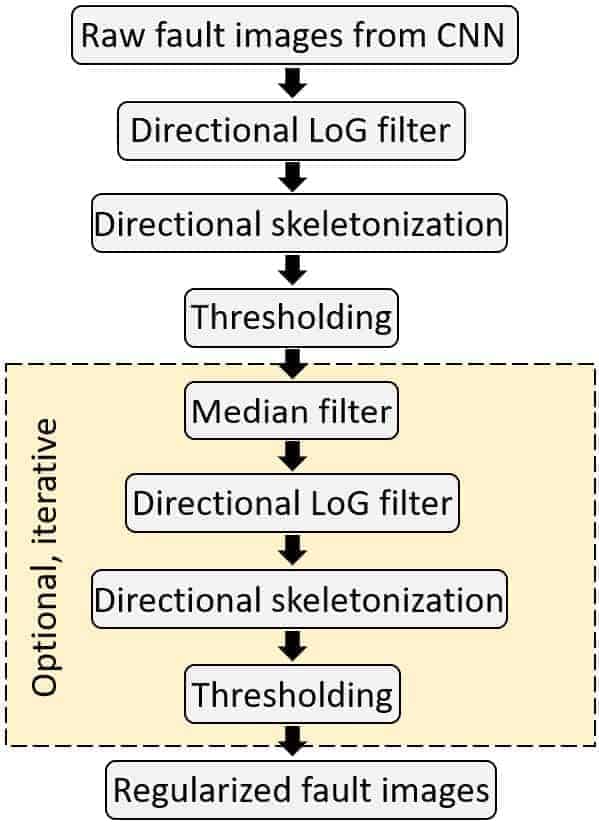
We then use a suite of image processing techniques to improve the quality of the fault images. First, we use a directional Laplacian of Gaussian (LoG) filter (Machado et al., 2016) to enhance lineaments that are of high angle from layering reflectors and suppress anomalies close to reflector dip, while calculating the dip, azimuth, and dip magnitude of the faults. Taking these data, we then use a skeletonization step, redistributing the fault anomalies within a fault damage zone to the most likely fault plane. We then do a thresholding to generate a binary image for faults. Optionally, if the result is still noisy, we can continue with a median filter to reduce the random noise and iteratively perform the directional LoG and skeletonization to achieve a desirable result. Figure 2 summarizes the regularization workflow.
Synthetic Test
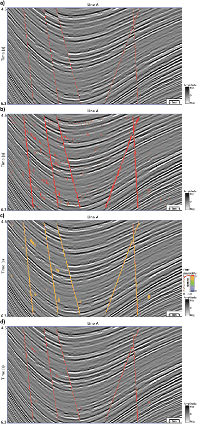
We first test the proposed workflow on synthetic data built on the SEAM model. To make the model a good approximation of real field data, we select a portion in the SEAM model where stacked channels and turbidites exist. We then randomly insert faults in the impedance model and convolve with a 40Hz Ricker wavelet to generate seismic volumes. The parameters used in random generation of five reverse faults in the 3D volume are provided in Table 1. Figure 3a shows one line from the generated synthetic data with faults highlighted in red. In this model, we observe strong layer deformation with amplitude change along reflectors due to the turbidites in the model. Therefore, such synthetic data are in fact quite challenging for a fault detection algorithm, because of the existence of other types of discontinuities.
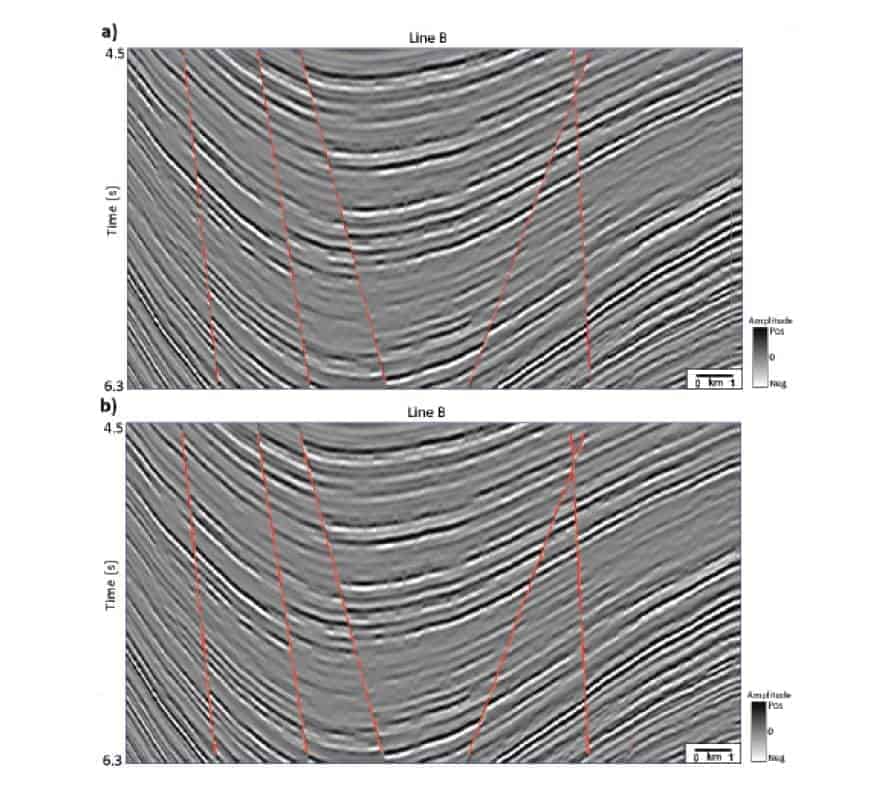
We randomly use 20% of the samples on the fault planes and approximately the same amount of non-fault samples to train the CNN model. The total number of training sample is about 350,000, which represents <1% of the total samples in the seismic volume. Figure 3b shows the raw output from the CNN fault detector on the same line shown in Figure 3a. We observe that instead of sticks, faults appear as a small zone. Also, as expected, there are some misclassifications where data are quite challenging. We then perform the regularization steps excluding the optional steps in Figure 2. Figure 3c shows the result after directional LoG filter and skeletonization. Notice that these two steps have cleaned up much of the noise, and the faults are now thinner and more continuous. Finally, we perform a thresholding to generate a fault map where faults are labeled as “1” and “0” for everywhere else (Figure 3d). Figure 4 shows the fault detection result on a less challenging line. We observe that the result on such line is nearly perfect.
| Fault attribute | Values range |
| Dip angle (degree) | -15 to 15 |
| Strike angle (degree) | -25 to 25 |
| Displacement (m) | 25 to 75 |
Table 1. Parameter ranges used in generating faults in the synthetic model.
Field Data Test
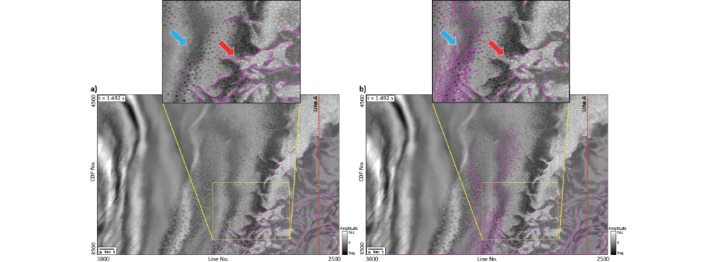
We further verify the proposed workflow on field data from the Great South Basin, offshore New Zealand. The seismic data contain extensive faulting with complex geometry, as well as other types of coherence anomalies as shown in Figure 5. In this case, we manually picked training data on five seismic lines for regions representing fault and non-fault. An example line is given in Figure 6. As one may notice, although the training data consist very limited coverage in the whole volume, we try to include the most representative samples for the two classes. On the field data, we use the whole regularization workflow including the optional steps. Figure 7 gives the final output from the proposed workflow, and the result from using coherence in lieu of raw CNN output in the workflow. We observe that the result from CNN plus regularization gives clean fault planes with very limited noise from other types of discontinuities.
Conclusion
In this study, we introduce a fault detection workflow using both CNN-based classification and image processing regularization. We are able to train a CNN classifier to be sensitive to only faults, which greatly reduces the mixing between faults and other discontinuities in the produced faults images. To improve the resolution and further suppress non-fault features in the raw fault images, we then use an image processing-based regularization workflow to enhance the fault planes. The proposed workflow shows great potential on both challenging synthetic data and field data.
Acknowledgements
The authors thank Geophysical Insights for the permission to publish this work. We thank New Zealand Petroleum and Minerals for providing the Great South Basin seismic data to the public. The CNN fault detector used in this study is implemented in TensorFlow, an open source library from Google. The authors also thank Gary Jones at Geophysical Insights for valuable discussions on the SEAM model.
References
Araya-Polo, M., T. Dahlke, C. Frogner, C. Zhang, T. Poggio, and D. Hohl, 2017, Automated fault detection without seismic processing: The Leading Edge, 36, 208–214.
El-Sayed, M. A., Y. A. Estaitia, and M. A. Khafagy, 2013, Automated edge detection using convolutional neural network: International Journal of Advanced Computer Science and Applications, 4, 11–17.
Fehler, M., and K. Larner, 2008, SEG Advanced Modeling (SEAM). Phase I first year update: The Leading Edge, 27, 1006–1007.
Huang, L., X. Dong, and T. E. Clee, 2017, A scalable deep learning platform for identifying geologic features from seismic attributes: The Leading Edge, 36, 249–256.
Machado, G., A. Alali, B. Hutchinson, O. Olorunsola, and K. J. Marfurt, 2016, Display and enhancement of volumetric fault images: Interpretation, 4, 1, SB51–SB61.
Marfurt, K. J., V. Sudhaker, A. Gersztenkorn, K. D. Crawford, and S. E. Nissen, 1999, Coherency calculations in the presence of structural dip: Geophysics, 64, 104–111.
Qi, J., G. Machado, and K. Marfurt, 2017, A workflow to skeletonize faults and stratigraphic features: Geophysics, 82, no. 4, O57–O70.
Waldeland, A. U., and A. H. S. S. Solberg, 2017, Salt classification using deep learning: 79th Annual International Conference and Exhibition, EAGE, Extended Abstracts, Tu-B4-12.
Wu, X., and D. Hale, 2016, 3D seismic image processing for faults: Geophysics, 81, no. 2, IM1–IM11.
Xie, S., and Z. Tu, 2015, Holistically-nested edge detection: Proceedings of the IEEE International Conference on Computer Vision, 1395–1403.

