By Rocky Roden | May 2020
Introduction to Machine Learning for Interpreters
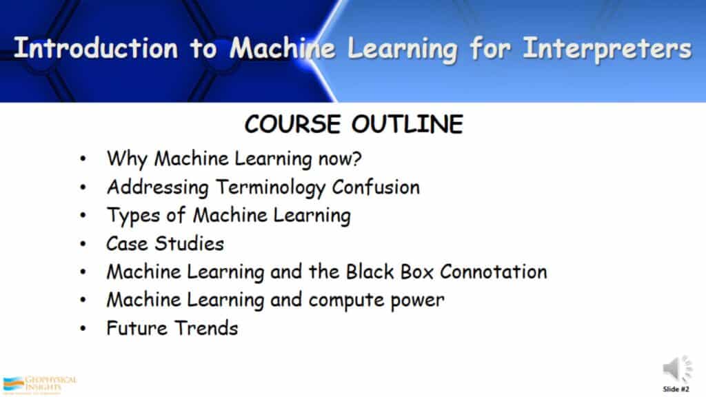
● Why Machine Learning now?
● Address terminology confusion
● Types of Machine Learning
● Case studies
● Machine Learning and the “Black Box” connotation
● Machine Learning and compute power
● Future trends
How does Machine Learning Relate to Finding Oil and Gas?
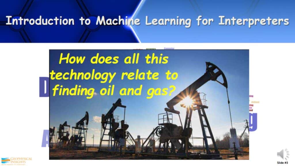
We hear a lot of words today in our lives related to machine learning, artificial intelligence, deep learning, which can be quite confusing at times. However, the focus of this webinar is “How does all this technology relate to finding oil and gas?”.
Why Use Machine Learning?
You may ask, “Why use machine learning now?” Well, machine learning is very good at helping to analyze large amounts of data simultaneously. It’s the Big Data issue.Machine learning can certainly help to determine the relationships between several types of data all at once. For example, in the interpretation process, we typically look at 2D and 3D crossplots. What happens when I have 5, 10, or even 20 different types of data. How do they relate or not relate to each other? Machine learning can help us in this regard. Machine learning can also help discover nonlinearities in the law of the solutions that we use now in the interpretation process. We quite often make assumptions on different elements of the Earth, when in reality they are not linear but very complicated. Quite often machine learning can help understand these nonlinearities. It can certainly improve the efficiency and accuracy over time and ultimately, it can help automate a lot of these interpretive processes. Overall, helping us to be more effective and efficient. Of course, the ultimate goal in machine learning is to help interpreters reveal geological features, properties, or trends that are very difficult to see or interpret in our data or the data unable to be seen with conventional approaches. Ultimately, it’s reducing the risk in drilling for oil and gas.
Challenges and Opportunities for Machine Learning in the Geosciences
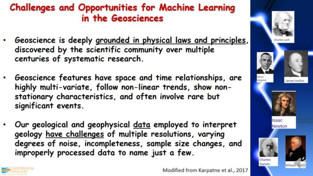
Geoscience is deeply grounded in physical laws and principles. These have been developed by many of the people seen pictured in the right, over multiple centuries of a lot of systematic research. Geoscience features have space and time relationships, highly multi-variate, follow many non-linear trends, lots of non-stationary characteristics, and often involve rare but significant events. Then the geoscience data itself can have challenges. These can include: multiple resolutions, varying degrees of noise, incompleteness, sample size issues, and improperly processed data, just to name a few.
Machine Learning in Geosciences
The questions are:
-How can geoscience interpreters ensure that the established bounds and rigorous theories, that have been established over centuries, are not violated by machine learning. By the same token, how can we advance our geoscience interpretation, especially with Machine Learning, if we are restricted by the established practices of the past? Well, the answer is pretty easy. In the Oil and Gas industry, the proof is what is found by the drill bit. That ultimately tells us the answers. It is obvious we don’t have all of the answers yet. If we did, no one would ever drill a dry hole.
Data Science vs Big Data vs Data Analytics
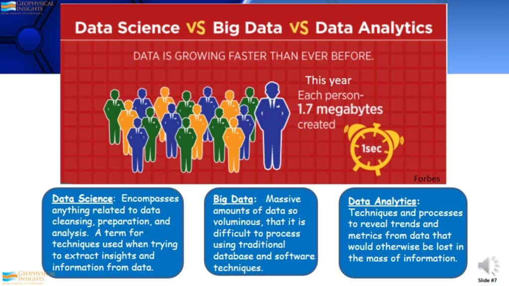
Forbes indicates that data is growing so fast that by this year, 2020, data will be growing at the rate of 1.7 megabytes per second, for every person on Earth. That is a tremendous amount of information. That is why the data science field has dramatically grown over the last decade. Data science encompasses anything related to preparing, looking at, or analyzing lots of data. The Big Data issue relates to having such massive amounts of data, that require other processes to evaluate it. Traditional database and software techniques don’t work anymore. Data analytics are just the approaches and techniques used to analyze all of this information.
What is Machine Learning?
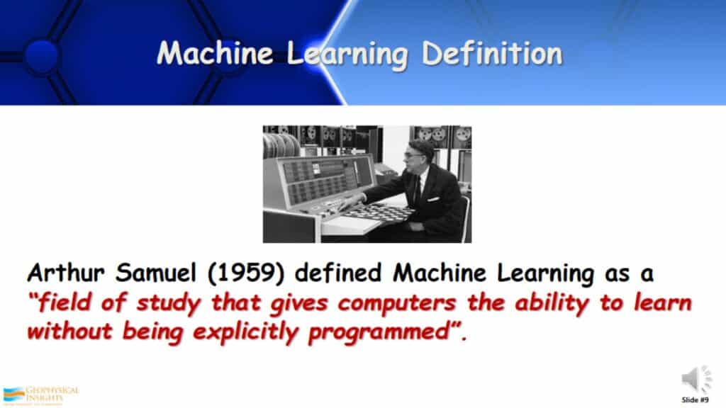
Most people give a definition of Machine Learning accredited to Arthur Samuel, who indicated it’s the “field of study that gives computers the ability to learn without being explicitly programmed”. We’ve heard a lot of the modern-day challenges of computer systems beating the chess champions of the world and other games. However, many people don’t realize Arthur Samuel developed an IBM machine that ran Machine Learning that beat the checkers champion of Connecticut. This is part of the evolution of Machine Learning.
Categories of Data Science
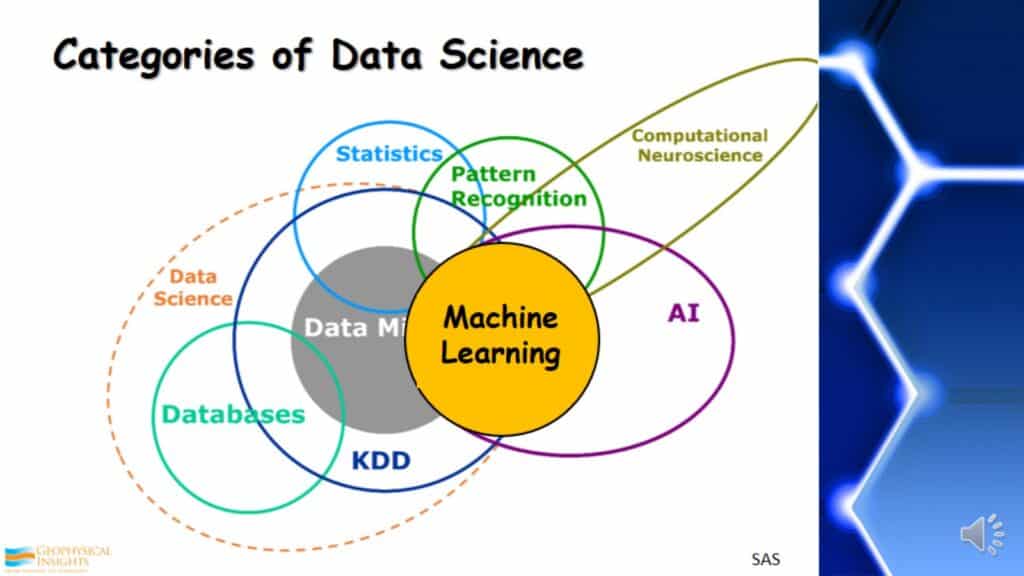
This display exhibits a lot of different categories of data science but, what’s important to look at is where Machine Learning is located in these sorts of data science categories. As shown, it is a part of AI (artificial intelligence).
Categories of Data Science – Artificial Intelligence
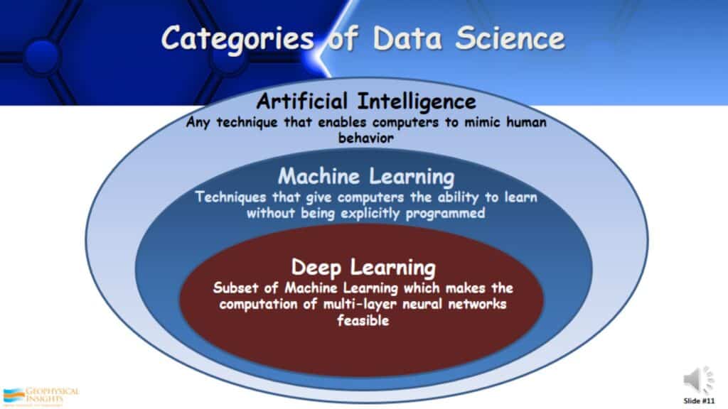
Artificial intelligence is a big and very significant category of data science. AI is any technique that enables computers to mimic human behavior. A subset of AI is Machine Learning. As defined by Arthur Samuel, it is a technique that gives computers the ability to learn without being explicitly programmed. A subset of Machine Learning is Deep Learning. That relates to the computation of multi-layer neural networks.
Types of Machine Learning
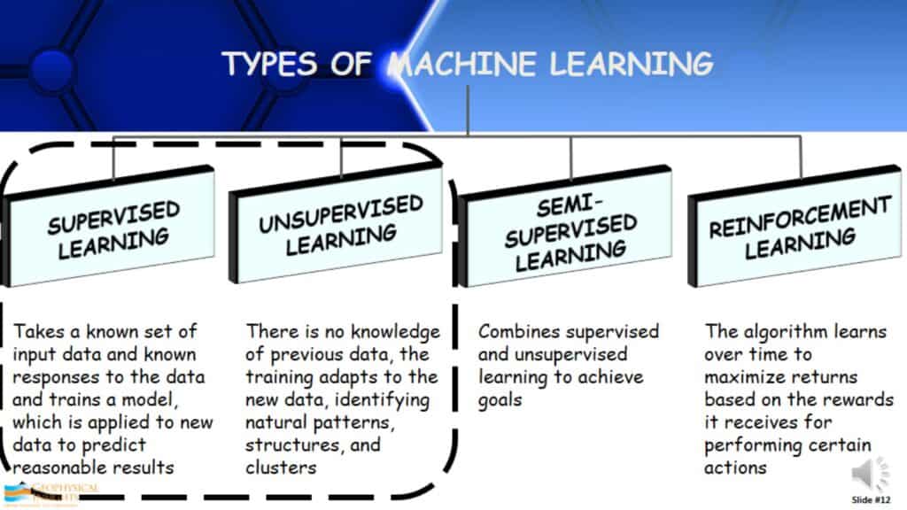
If you were to Google Machine Learning, you’d get something similar to the following:
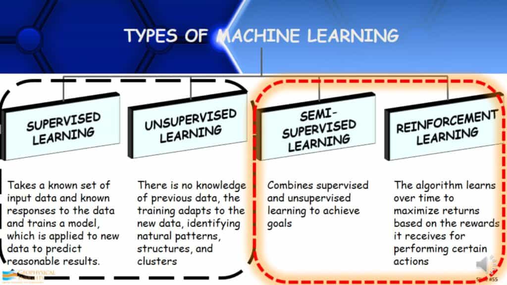
Supervised Learning- It is the most widely used type of machine learning. It takes a known set of input data and the known responses, and then takes the description/label that it describes and then develops a model to find the answer that is already known. Once the model is developed, it can be applied to another data set hoping to find what was originally found when developing the model.
Unsupervised Learning- It is actually quite different. In unsupervised learning, there is no knowledge of previous data. The training adapts to the data, identifying natural patterns, structures, and clusters. A great example is babies. Most researchers think that newborn babies, up until about a year old, fundamentally learn by unsupervised learning. They come into this world not knowing anything other than their surroundings, items in the surroundings, and parents. They look at the relationships of the things around them.
Semi-Supervised Learning- It is really combining supervised and unsupervised learning in different ways to get better answers.
Reinforcement Learning- This is the type of algorithm that learns over time and maximizes returns based on the rewards it receives for performing certain actions.
We will focus mainly on supervised and unsupervised learning, how it’s being used, and a few examples of interpreting geology. Semi-supervised and reinforcement learning will be discussed later in the presentation.
Supervised and Unsupervised Machine Learning
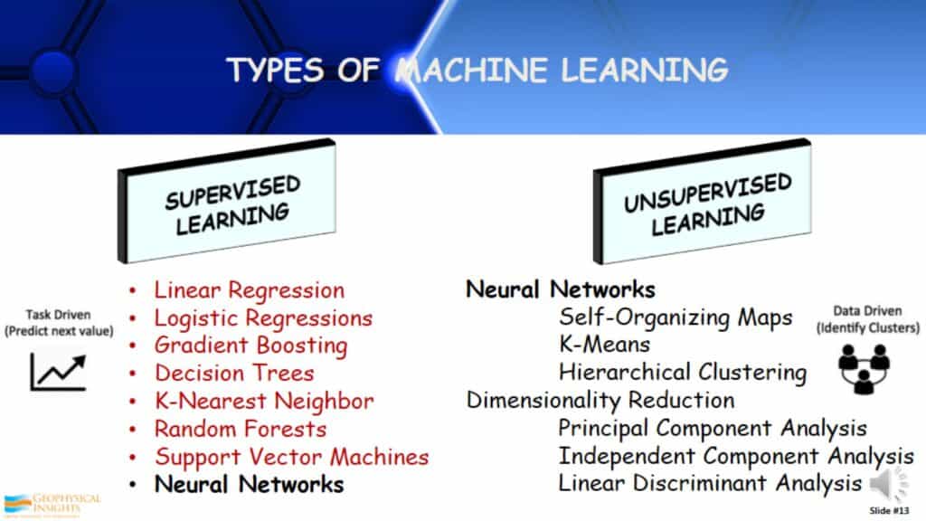
There are many types of supervised and unsupervised learning. Listed are some of the different kinds of machine learning approaches that are seen and used in the Geoscience community for interpretation. The left list (unsupervised learning) are a few very common approaches in geological applications. Approaches listed in red are non-neural network statistical approaches. Of course there are neural networks under unsupervised learning. Over in unsupervised learning, there neural networks again. Different than the ones in supervised learning along with something called dimensionality reduction. This will be discussed as it relates to unsupervised learning.
Non-Neural Network Machine Learning (Regression and Classification)
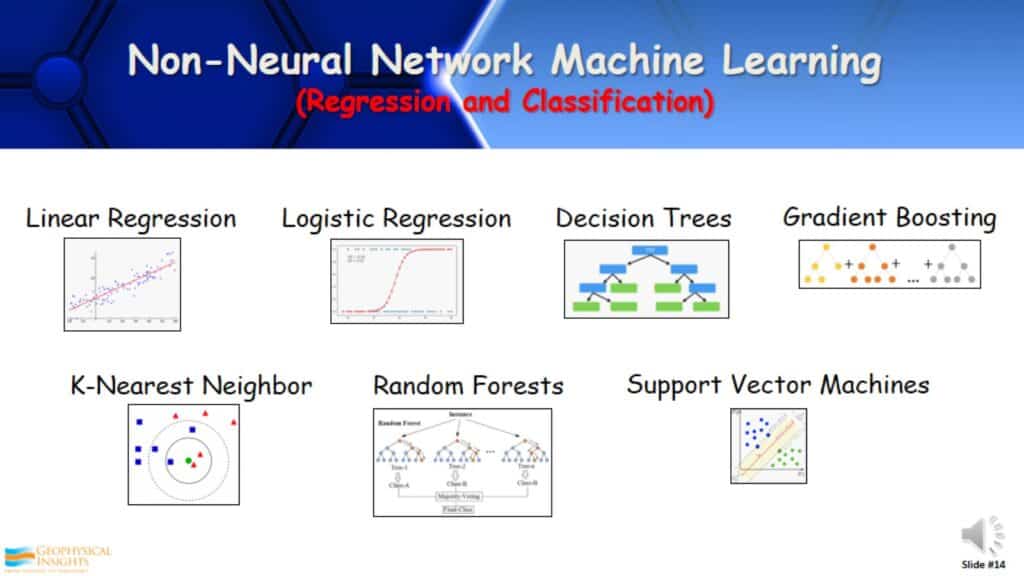
Of these non-neural networks supervised learning approaches like linear regression, decision trees, and random forests. These are all regression and classification approaches to help solve some interpretational problems. I’ll give some examples.
AVO intercept and gradient computed from least-squares linear-fit line (Linear Regression) through amplitude vs Zoeppritz approximation
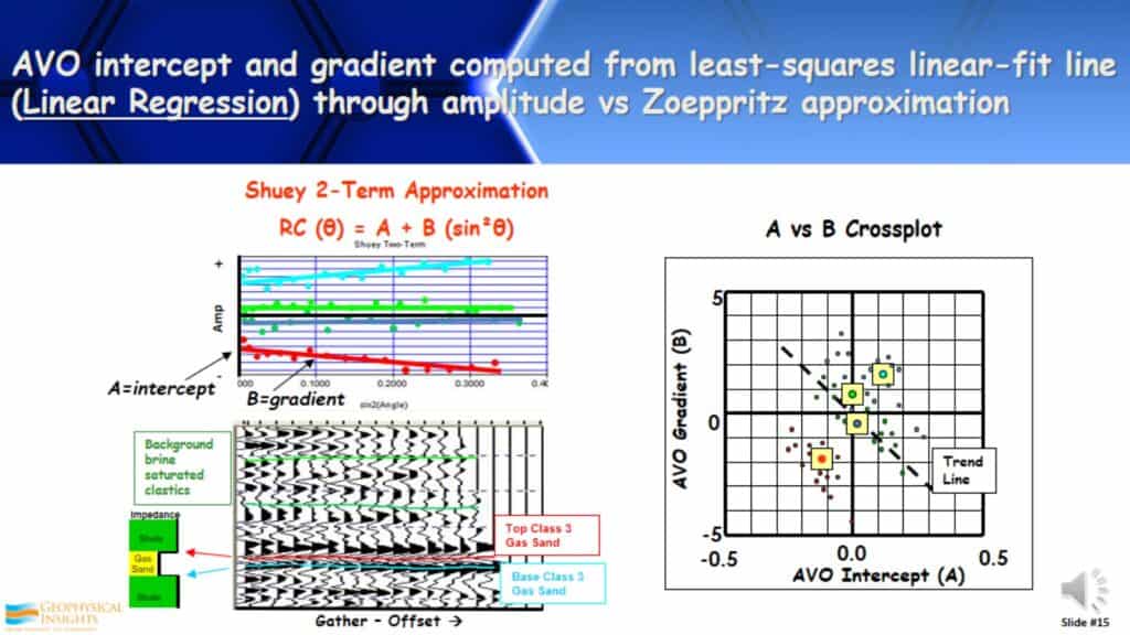
Being an AVO guy, one of the things that I have been doing for years, and anyone that interprets AVO will be familiar with, is calculating intercepting gradients. It’s a very simple linear regression when calculating how amplitudes change with offset depending on what kind of linear approximation being used. For example, here is a Shuey 2-Term. I crossplot that and do a least-squares linear-fit line. The slope of that line is a gradient and the intercept is a zero offset. Those are two of the fundamental attributes used in our industry. Linear regression; very simple and very straight forward.
Comparison of Acoustic Impedance Inversion and Predictive Analytics to determine key reservoir properties for 4D surveys
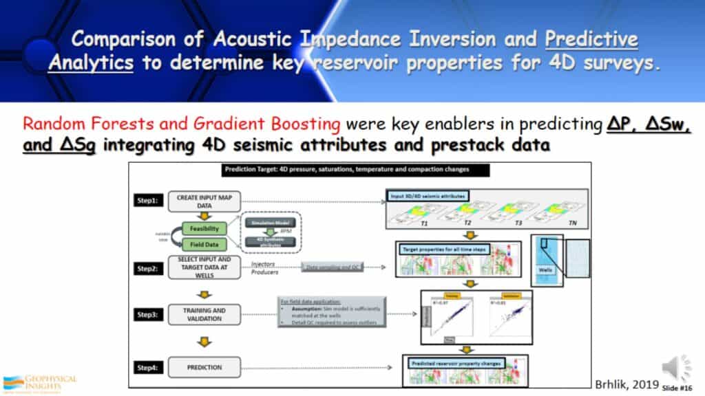
Another approach of non-neural networks in supervised learning is by ConocoPhillips. They did an analysis of their 4D surveys in the Gulf of Mexico and North sea. They came to the conclusion that the Acoustic Impedance Inversion they were using, was not sufficient enough to see the changes in the reservoir properties that they wanted to see. As a consequence, they applied Random Forests and Gradient Boosting along with 4D seismic attributes and prestack data. This apparently enabled them to much better predict the change in pressure, water saturation, and gas saturation. Again, this was by using some non-neural network supervised learning approaches.
Neural Networks
Neural networks are obviously a very popular and common approach of Machine Learning to use in interpreting geology and geophysics.
Biological Neural Network
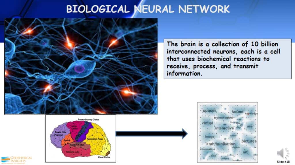
A lot of neural networks are based on the biological neural network. This relates to the brain, which is a collection of 10 billion interconnected neurons. Each of these cells uses biochemical reactions to receive, process, and transmit information.
Artificial Neural Network
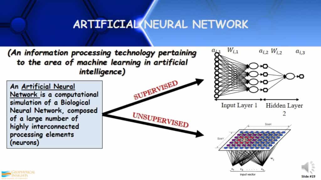
An Artificial Neural Network is no more than a computational simulation of a Biological Neural Network. It’s composed of a large number of highly interconnected processing elements, called neurons. Here we have both supervised and unsupervised with neurons being used very differently in both. The computations are very different.
An Example of Supervised Learning
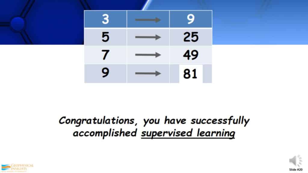
Here is a test for you. Look at these series of numbers. Based on these numbers, what is the answer to the missing number? Hopefully you got 81. Congratulations, you have successfully accomplished supervised learning. You looked at the series of numbers, you built a model that relates to squaring the first number to get the number on the right, applied this to the test at the bottom, and got 81. This is a typical example of supervised learning.
Supervised Learning – Neural Network
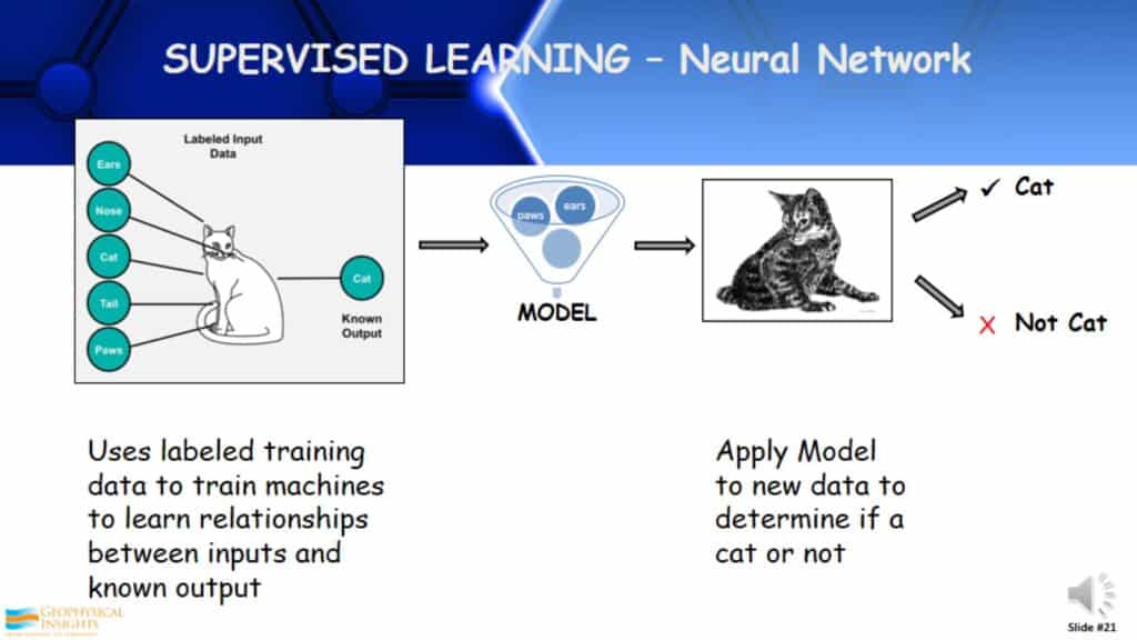
How supervised learning works; I take a known object. For example, here we have my cat and a description of it, which are sometimes called labels. Ultimately, I develop a model that determines this is a known cat. I take this model and apply it to another object, and it determines whether the object is a cat or not. This is fundamentally supervised learning.
Supervised Learning – Pros & Cons
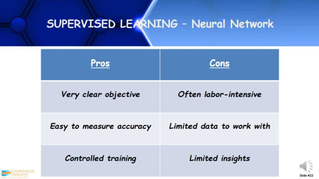
What are the pros and cons of supervised learning? Pros: It’s a very clear objective. This is why it’s the most used Machine Learning application today. It is easy to measure the accuracy and it is controlled. Cons: It can be labor-intensive, especially if you’re trying to develop the labels or descriptors. Do you have enough information to really build an accurate model? It fundamentally gives you limited insights, because you’re telling it what to find. It won’t find anything that you don’t tell it to find.
Deep Learning/Deep Neural Network – More that one hidden layer
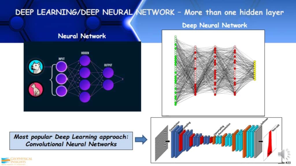
Another aspect of supervised learning is in the neural network. If you look to the left, this is a very simple neural network, sometimes called a shallow neural network. You have the input (which is the labels/descriptors), you have one hidden layer of neurons, and then you have the output. If you look on the right, this is a deep neural network, sometimes called deep learning. There are several hidden layers there, in this case, there are a lot of neurons in each layer. The most popular deep learning approach today, on the bottom, is a Convolutional Neural Network (CNN). CNNs were developed out of image recognition. It takes an image input and assigns weights and biases to differentiate one from the other.
Supervised Learning Case Study
Deep Learning – Convolutional Neural Network
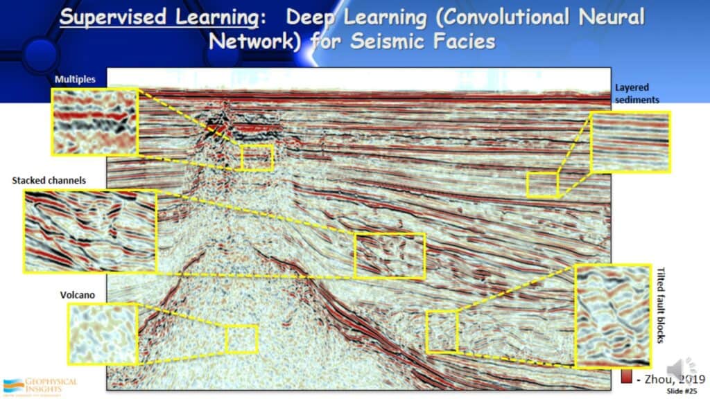
In this example, there is a seismic line and I am going to identify seismic facies. What I typically do is look at several lines in a 3D survey and identify reflection patterns on those lines that I want to be interpreted throughout the entire dataset. By identifying these patterns. T starts to build a model A model that recognizes these different reflection patterns, hopefully in many cases associated with seismic facies.
Deep learning for seismic facies classification
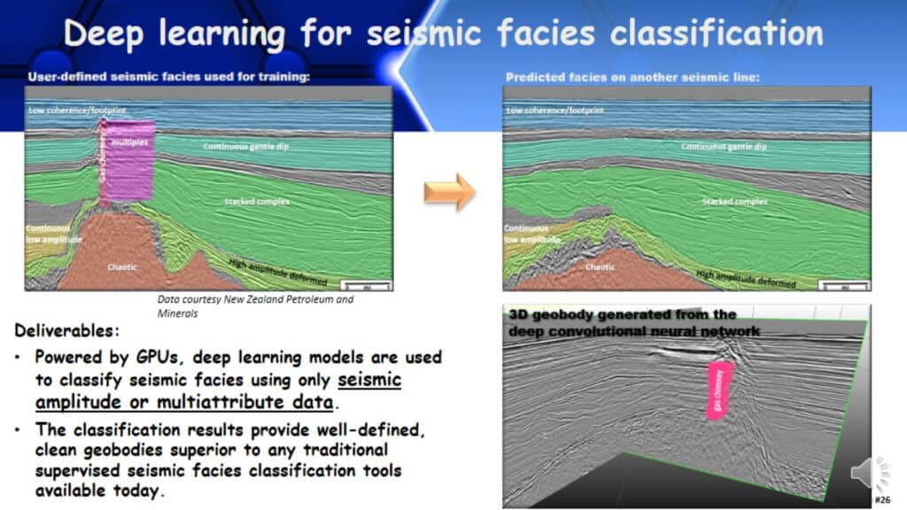
Typically these are generated or run on graphic processing units (GPUs). It looks at the data, takes this model and analyzes all the data based on the few input lines given to build the model, then it classifies the whole dataset.
3D Visualization of the Facies Classification
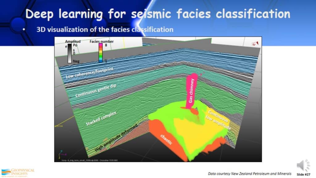
Once it’s done you have a 3D visualization of the facies you originally wanted to see in your data. This is an example of a Convolutional Neural Network for seismic facies interpretation.
How Many Patterns or Clusters Can You Identify?
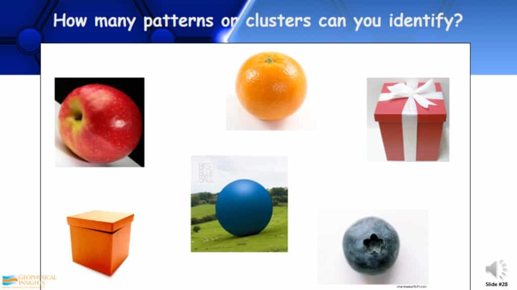
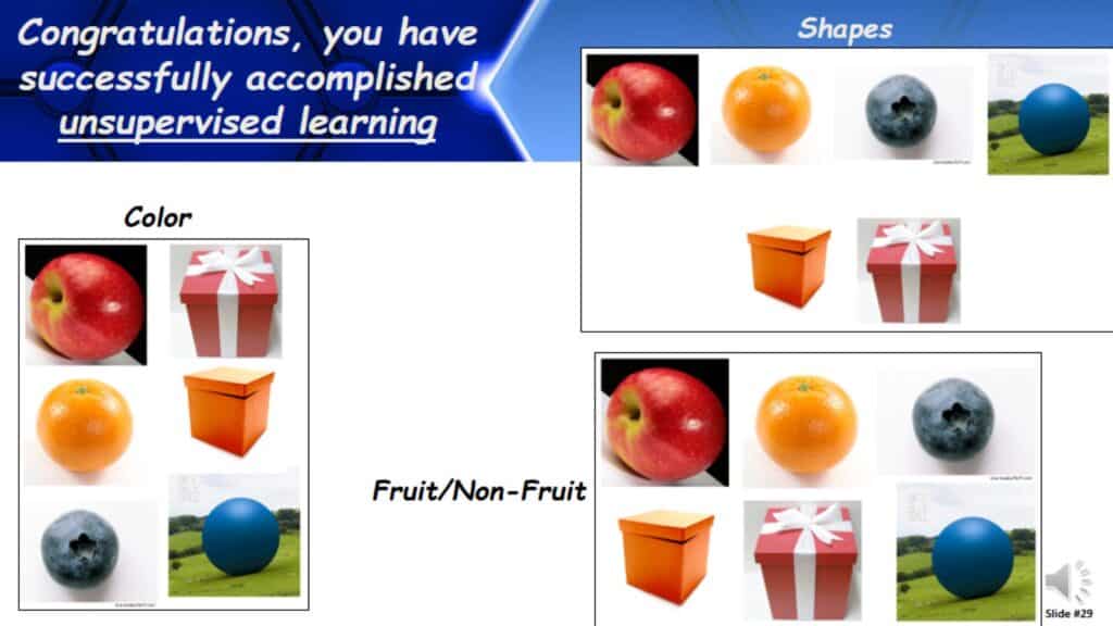
Here is another test. How many patterns or clusters can you identify from these six objects? Look at these and think about this. Shapes, Fruit/Non-Fruit, Color, and etc. Congratulations, you have successfully accomplished unsupervised learning. Very different, here you were looking for the natural patterns or clusters. How did you identify them?
Unsupervised Learning
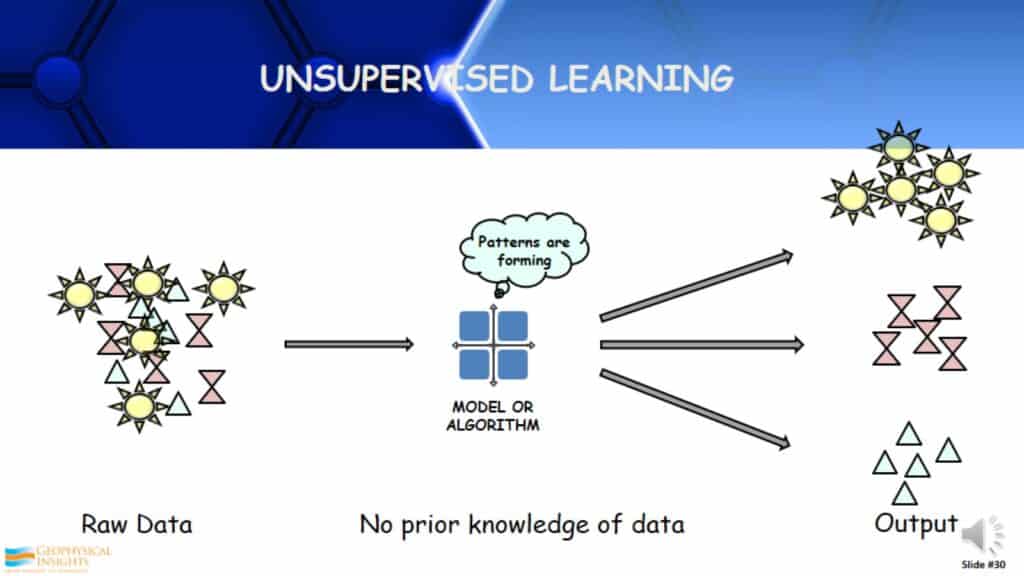
How does unsupervised learning work? You take a large amount of raw data that you know nothing about and apply an unsupervised learning algorithm. It examines the data, learns from the data, and identifies the patterns/clusters/classes. Then it separates that out into different patterns. The thing that is different about unsupervised learning, is you have to interpret those patterns, unlike supervised learning where you knew what you were trying to find. You may or may not understand what you ultimately get out of unsupervised learning.
Unsupervised Learning – Neural Networks
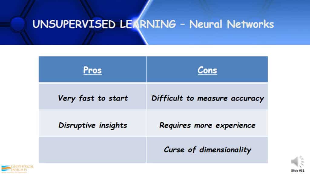
Here are the pros and cons of unsupervised learning. Pros It is very fast to start. I don’t need a lot of descriptors or labels going into the process. It can be very disruptive, it may show you things you have never seen before or didn’t understand. Cons: It is somewhat difficult to measure the accuracy. It does require a little bit more experience on the perimeters quite often. There is another issue of something called the curse of dimensionality.
Curse of Dimensionality
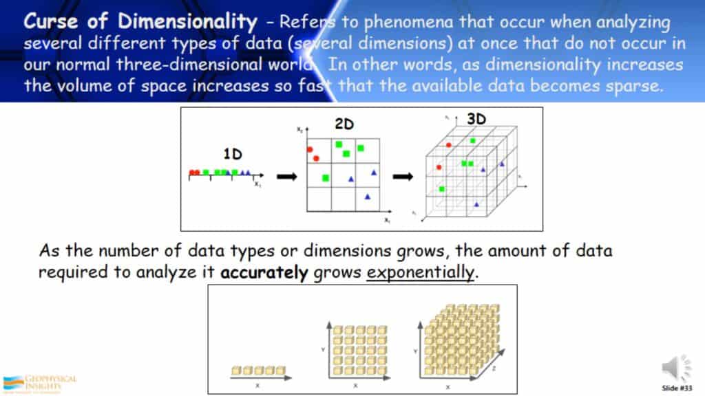
The curse of dimensionality is a phenomenon quite often associated with unsupervised learning. So what does this mean? It refers to a phenomenon that occurs when analyzing several different types of data, in other words several dimensions, at one time. There are issues that come up that are not related to the normal 3D world that we live in. In other words, as the amount of data or dimensionality increases, the volume of space increases so fast that the available data becomes sparse. What does this mean? Take for example the 1D plot seen on the bottom. You see a series of data points on the 1D graph. If you take those same points and plot them on a 2D graph you see they start to space in between the data points. If you take the 3D graph, on the right, you have a lot more space between the points. As the number of data types or dimensions grow, the amount of data required to analyze it accurately grows exponentially.
How to defeat the Curse of Dimensionality?
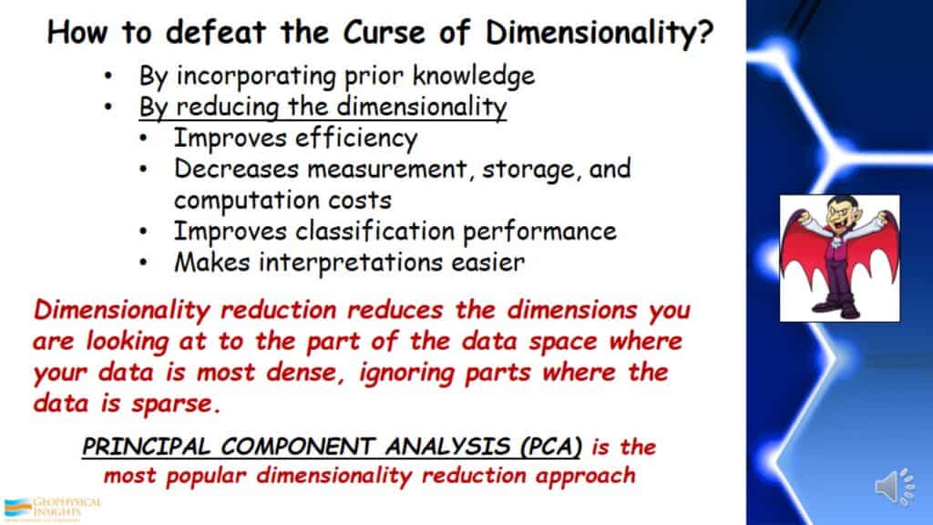
How do we defeat the Curse of Dimensionality? The first way is by incorporating prior knowledge. Then we need to reduce its dimensionality. This needs to be done to improve classification performance and make interpretations feasible. Dimensionality reduction reduces the dimensions you are looking at to the data space where your data is most dense, ignoring parts where the data is sparse. One of the most common and popular approaches used today to reduce dimensionality is Principal Component Analysis (PCA).
Principal Component Analysis (PCA)
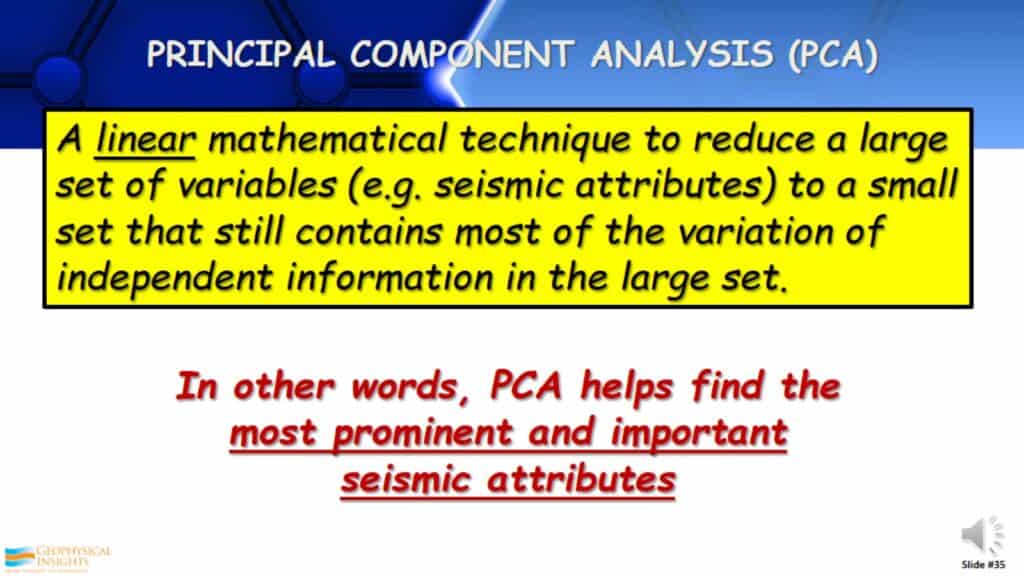
This is a linear mathematical technique to reduce a large set of variables (e.g. seismic attributes) to a small set that still contains most of the variation of independent information in the large set. This means it can help us find the prominent attributes in the dataset.
What is the Largest Variation in the Data?
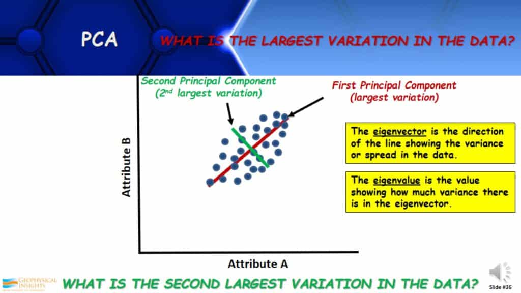
Here is a graphic approach to understanding principal component analysis. If I were to crossplot a couple of attributes and the data looked as the information in the graph below, what is the largest variation in the data? You can see that the largest variation or spread of data is shown by the red line. This is the first PCA. What is the second-largest variation in the data? There are two attributes and two principal components. The second one is orthogonal to the first and it shows the second-largest variation in the data, shown by the green line. The eigenvector is the direction of the line sowing the variance or spread in the data. The eigenvalue is the measure of that variance. How does this relate to interpreters?
PCA in Twelve Seismic Attributes
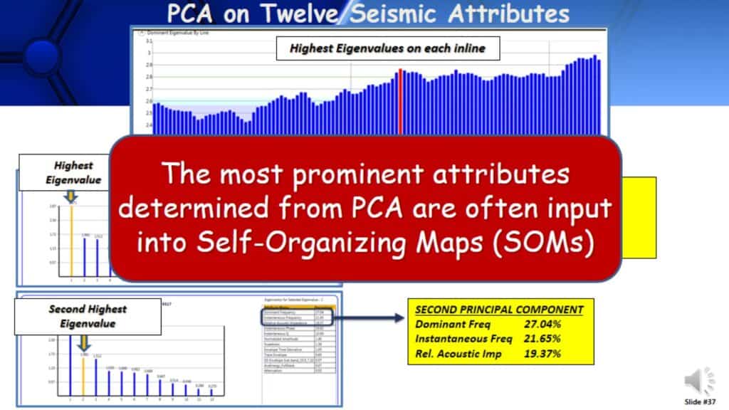
Here is an example of principal component analysis. Here we have taken twelve seismic attributes and one PCA. The graph depicts the highest eigenvalues on each of the inlines in this 3D survey. So for example, if I took the red bar and wanted to look at the PCA as it relates to the red bar, say this line was running directly through the well of interest. These are the results, twelve attributes, and twelve principal components. The first principal component, which is the highest eigenvalue, there are twelve attributes listed and highlighted is the percentage contribution. There are four attributes that stand out with over 90% contribution of the first principal component. There is no question that these four attributes are very prominent in the data. The second principal component has three prominent attributes in the data. Looking at the first and second principal components there are seven attributes that are very prominent in the dataset. Those attributes can be taken and take them into an unsupervised approach such as Self-Organizing Maps (SOMs). The real issue is, are these the attributes to uncover that I am looking for?
Self-Organizing Maps (SOMs)
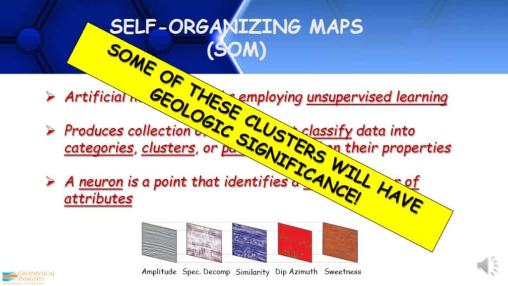
Self-Organizing Maps (SOMs) are an unsupervised learning approach. It classifies data into clusters, categories, or patterns based on their properties. A neuron is a point that identifies a natural cluster of attributes in the data. Some of these clusters will have geologic significance. Some of them will not; they will identify coherent/incoherent noise and other elements in your data that are not cared about. Although, as long as the right attributes are selected within the realm of reasonable and good data.
How SOM Works
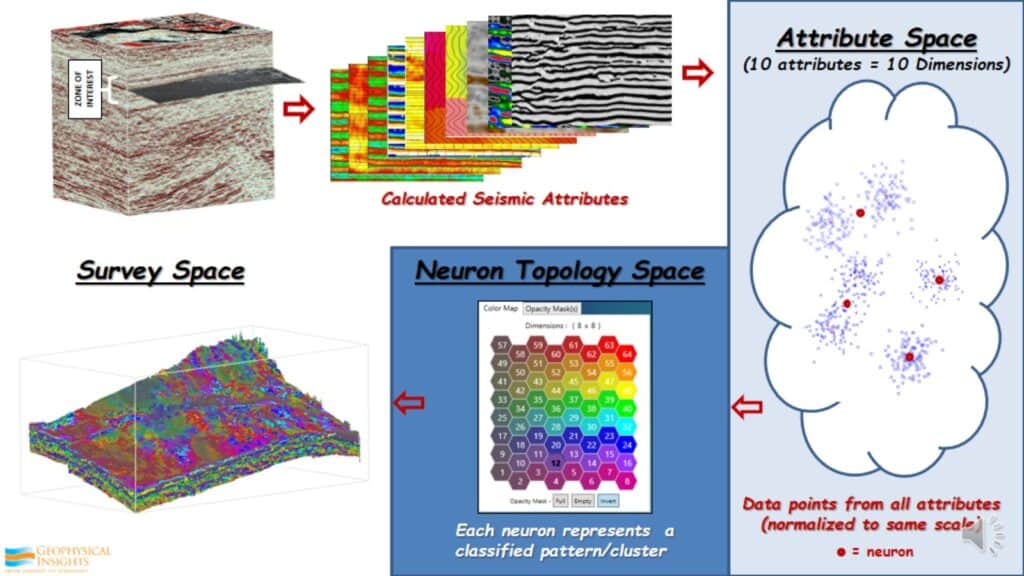
This is not too difficult. For example, there is a dataset with a very specific and identified zone of interest to be analyzed. There 10 prominent attributes in this dataset, within the zone of interest. What I do is take every one of these 10 attributes in that zone of interest, which means every single data point in that zone has 10 values. I take all of those of those data points and place them into attribute space. Initially, I was in survey space. Now I’ve calculated these attributes, taken all these data points, and put them into something call attribute space, sometimes called hyperspace. Because there are 10 attributes, there are 10 dimensions. That can not be seen visually, because there are 10 different data types. First thing I do is take all of those data types and normalize or standardize them to the same scale. Once that is done I will place neurons, in this case 64 neurons, randomly in this attribute space. Then I instruct the Self-Organizing Map to find the pattern in the data. The data points never move. The neurons move around, with very simple math, until it identifies 64 patterns in the data. Once it’s done that, it non-linearly maps this back to a Neuron Topology Space. In other words, as you are looking at the 2D color map there are 64 hexagons. Each one represents a neuron. Each neuron represents a pattern in the data that contains different percentages of the 10 attributes that went into it into the first place. This is how we take the information through the SOM classification process and go back to survey space. Now each one of the neurons that identify by color, show up in the 3D survey space so interpretations can be made. I can turn anyone or sets of neurons on or off to see whatever geology those particular neurons bring out in the data.
Unsupervised Learning Case Study
Principal Component Analysis and Self-Organizing Maps
Offshore Gulf of Mexico Case Study – Class 3 AVO
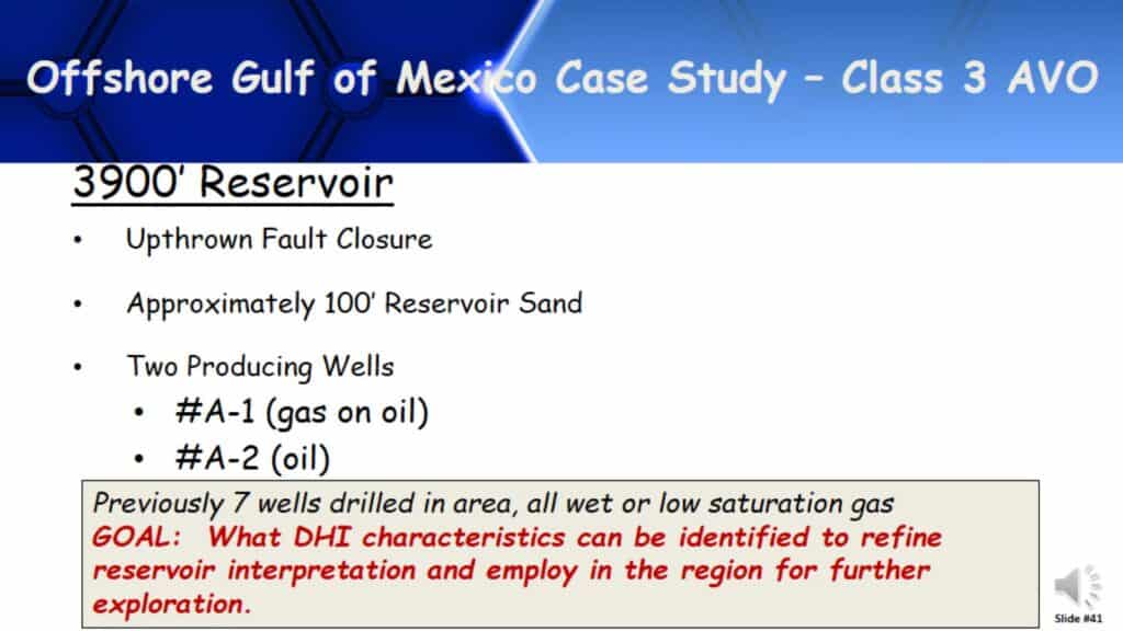
This case study is in the offshore Gulf of Mexico, a very simple Class 3 AVO Bright Spot setting. We are looking at a relatively shallow reservoir, for amplitudes and something that perhaps relates to DHIs, that can reduce the risks of drilling prospects in this area. Before these two wells were drilled, there were seven wells drilled in this area. All on amplitudes and all wet or low saturation gas, before these two wells made discoveries.
Attributes Input for PCA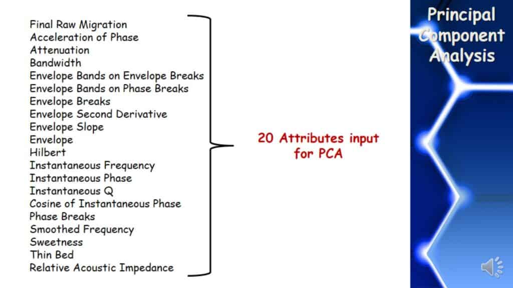
This data’s zone of interest took 20 instantaneous attributes in the Principal Component Analysis to find out what were the prominent attributes.
Principal Component Analysis
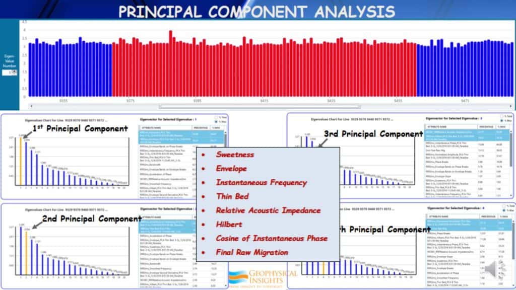
After taking these 20 seismic attributes and running through principal component analysis, here are the results. As you can see across the top, these bars represent the highest eigenvalue in each of the inlines of this particular survey. Now selecting the area where the red bars are located and the PCA results below are the average of each of the red bars in total. Then we look at the 1st, 2nd, 3rd, and 4th Principal Components, for the highest contributing attribute in each of the four principal components. The highest percentage of attributes as a whole, came out to be these eight attributes: Sweetness, Envelope, Instantaneous Frequency, Thin Bed, Relative Acoustic Impedance, Hilbert, Cosine of Instantaneous Phase, and Final Raw Migration. These eight attributes were placed in Self-Organizing Maps.
SOM Attributes and Analysis
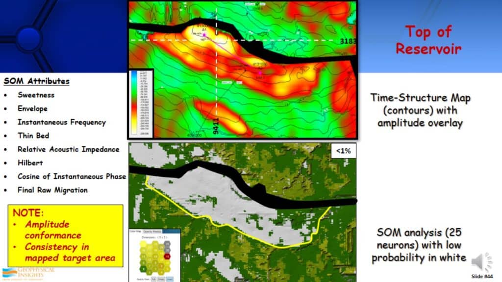
The top display is a map of the amplitude, the top of the reservoir. It’s a very prominent and high amplitude event. There is a good amplitude conformance to structure, it’s relatively consistent in the mapped target area. The bottom display is a result form the Self-Organizing Map analysis. You will see low probability in white. Low probability is a measure of the probability of the data points and how close they are to the neuron that identified that particular pattern or cluster that they’re in. For example, there is a neuron that has identified a cluster or pattern. All the points that are very close to the neuron has a high probability, but the points that are very far away have a low probability. They are anomalous. What is anomalous in the seismic data? One of them is DHIs, direct hydrocarbon indicators, by definition of seismic anomalies. What we have found is quite often these low probability anomalies from SOM analysis, relate to direct hydrocarbon indicators. This depends on the geological setting you are in and the attributes being used. By comparing the displays, you will see the low probability, in this case less than 1% probability was clearly defining the lateral extent of the reservoir.
Stacked Amplitude and SOM Analysis of Line 9411
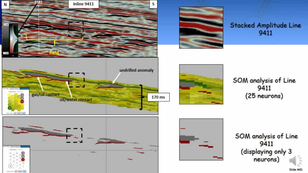
If you look at it from the standpoint of analyzing the neurons on the patterns they specifically see, this is the result. There is an inline right through the middle of the field. The top display is a typical conventional amplitude line in time through that field. The bottom two displays are the SOM results. If you pay attention to the middle display, you will see there are 25 neurons used there. The 20th and 25th neurons are identified in gray and if you look to the seismic line, the gray represents that reservoir above the hydrocarbon contacts. The hydrocarbon contacts are identified by the reddish color on neuron #15. It identified a gal/oil contact, oil/water contact, and something anomalous down deep that has not been drilled yet. The bottom display shows only those three neurons turned on. The dashed box on each display shows where the reservoir transitions from a hydrocarbon leg into a water leg. Looking at the SOM analysis you can see we are getting down to one or two samples where the reservoir pitches out and goes into the water leg; a much higher resolution than you normally see on seismic data.
Stacked Amplitude and SOM Analysis of Line 3183
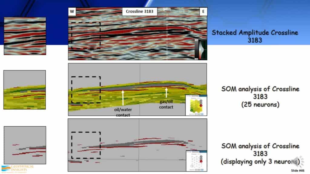
This is the same SOM display with a different focus. We are now looking at the strike line through that field. Again, look at the SOM results. You can see that reservoir identified by the two neurons in gray and the gas/oil contact identified by the reddish line. Very good identifying DHI characteristics in this particular dataset.
What is Machine Learning?
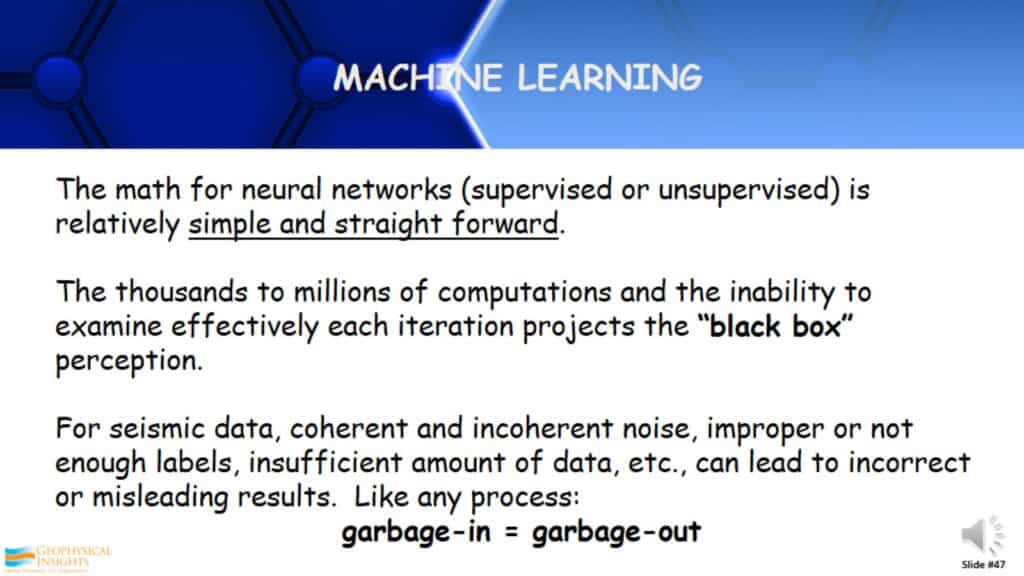
Machine Learning, whether you are using supervised or unsupervised methods, is relatively straightforward. In fact, many of the complicated mathematical derivations used in processing are quite involved. They are much more complicated than the neural network approaches used in machine learning. However, the difference is there are thousands of millions of computations involved in these neural networks. It is the inability to examine each of the iterations that projects the “black box” perception or connotation. Data goes in, there is an analysis, and data comes out with the answer. It is very difficult to understand how it got that answer because of so many computations. For seismic noise, coherent and incoherent noise, an insufficient amount of data, and etc can complicate this issue. It is this “black box” phenomenon at times that has prevented people from accepting some of the results. The computations at times can be quite compelling.
Machine Learning and Human Behavior
In Machine Learning (neural networks) we are typically trying to mimic human behavior by using inputs and receiving outputs. From the perspective of a machine learning system, the human is the black box. How do they come up with those answers?
Machine Learning and Compute Power
In Machine Learning, especially with neural networks, computing power has come to be a factor. Typically with Machine Learning, issues are based around things like CPU vs GPU, High-Performance Computing, and the Cloud.
Machine Learning and Compute Power – CPU & GPU
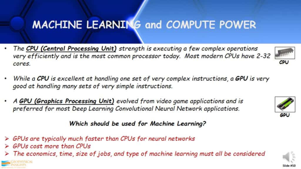
CPUs (Central Processing Units) which we all know are essential in all of our computers, are good at efficiently executing a few complex operations. While a CPU is excellent at handling one set of very complex instructions, a GPU (Graphics Processing Unit) is very good at handling many sets of very simple instructions. GPUs evolved from the gaming industry and it is a preferred approach for most Deep Learning Convolutional Neural Networks. Which should be used for Machine Learning? GPUs are typically faster than CPUs for neural networks. However, GPUs cost more than CPUs. Economics, time, size of the job, and machine learning types should all be considered. Often the Machine Learning applications will already be written for a GPU or CPU.
Machine Learning and Compute Power – HPC
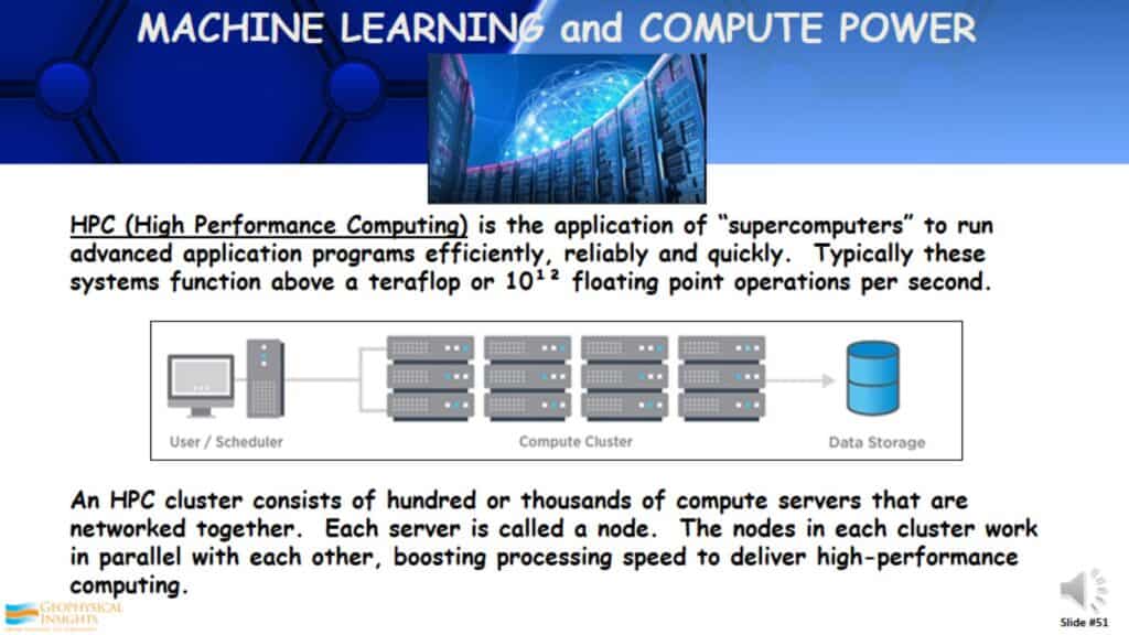
Another way Machine Learning is computed is by using HPC (High-Performance Computing) systems, sometimes called “supercomputers”. These HPC clusters consist of hundreds of thousands of compute servers that are networked together. Typically they are clustered and parallel with each other, boosting the processing speed, to give you a lot of high-performance computing. Of course, this is at a price.
Machine Learning and Compute Power – The Cloud
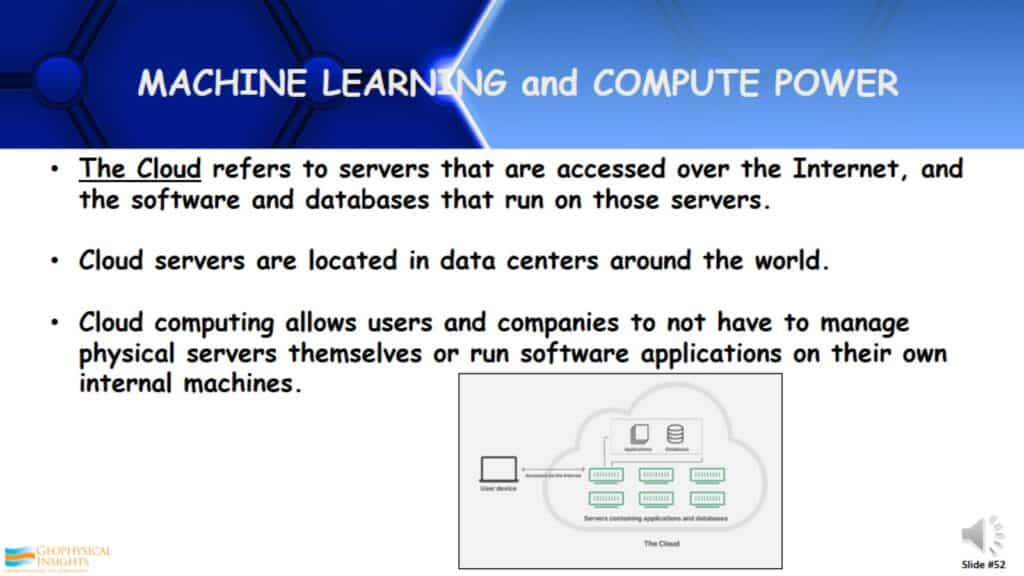
The Cloud refers to the servers that are accessed over the Internet and the software and databases that run in those servers. It could be a high-performance computing system or just a server you are using for computing. Whatever it is, you can have any with a Cloud. Cloud servers are located around data centers around the world. It allows companies and users to not have to manage physical servers themselves or run software applications on their own internal machines. All of this comes at a price, obviously.
Machine Learning Applications Being Developed Today
The majority of Machine Learning approaches today have been applied to our established geoscience workflows and practices. In other words, we are trying to improve elements of the traditional workflow. Can Machine Learning discover something “profound” that we have not seen before?
Profound Results from Machine Learning
University of Ontario Study
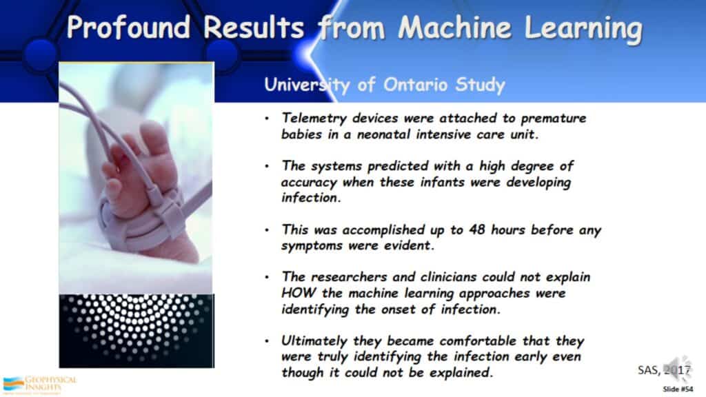
A study was done at the University of Ontario, where they looked at babies in an intensive neonatal care unit. Telemetry devices were attached to the babies. The purpose was to try to accurately identify when these babies were developing infections, one of the biggest worries for premature babies. This information was sent into a Machine Learning algorithm 48 hours prior to any symptoms becoming evident, that they would have infections. The process was becoming so good at identifying this that the doctors and clinicians believed what they were seeing, because of it’s high accuracy. They could not explain why the answers were being provided before they could see any symptoms. Of course there is a scientific explanation for this, however, they didn’t know what that was. It proved itself many times over. This is profound. It discovered something new and unknown.
Types of Machine Learning
With these different sorts of machine learning, which one of these might provide one of these profound step changes in how interpretation is done. We have discussed supervised and unsupervised learning. Supervised learning is one of the common Machine Learning applications used in our industry. Unsupervised Learning is less used, but this may provide us with profound step changes. It is able to produce disruptive changes that have never been seen before, unlike Supervised Learning where I am telling it what to find. In reality, the biggest advances will probably be in the Semi-Supervised and Reinforcement Learning approaches.
Semi-Supervised Learning
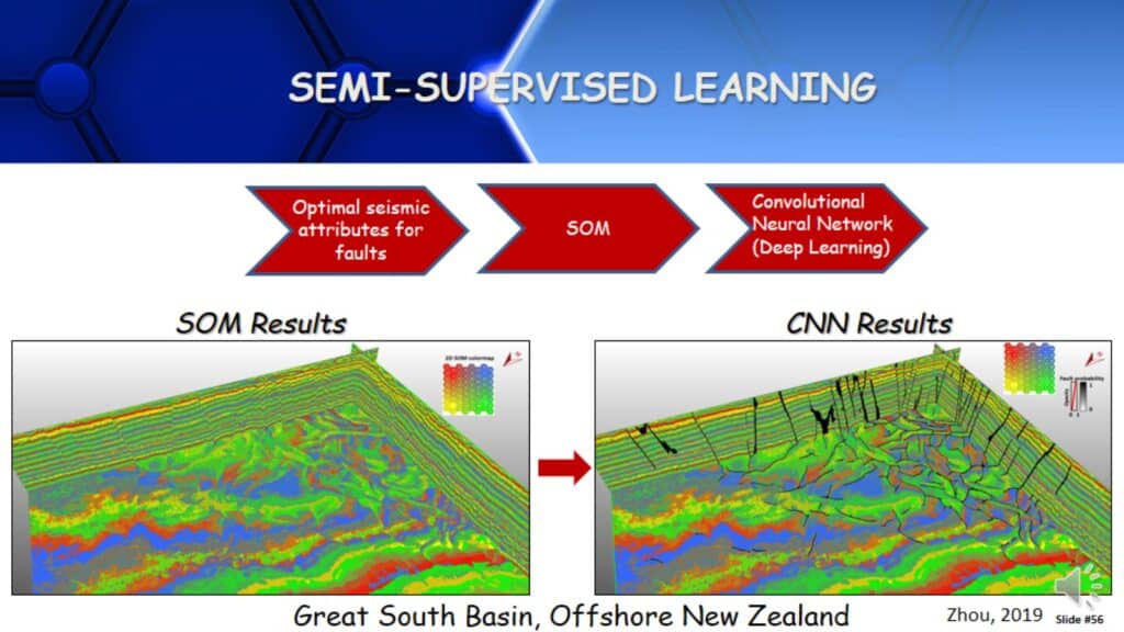
Here is an example of semi-supervised learning, which is really combining supervised and unsupervised learning approaches. For example, if I have gone through an unsupervised learning methodology, I have identified a set of attributes that are really good for faults. (i.e coherency, curvature, and etc.) Using those attributes, run a Self-Organizing Map, which is an unsupervised approach, and use those results in a Convolutional Neural Network that identifies faults. CNN is another deep learning approach. I have used two types of Machine Learning approaches with better data going in than conventional amplitude data to identify faults. This is a semi-supervised learning approach.
Will Machine Learning “Profoundly” Change Geoscience Interpretation?
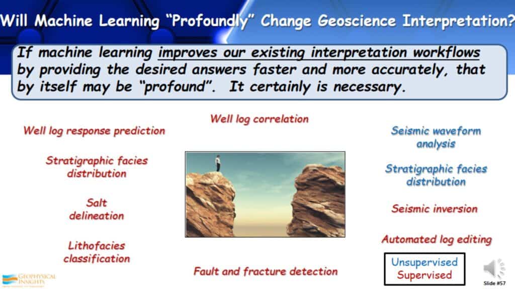
So will Machine Learning really change how we do interpretation? If machine learning improves our existing interpretation workflows by giving faster and more accurate answers, that in itself is significant and maybe “profound”. It is necessary, we have to be able to do things more efficiently, in less time, and with fewer people. Here are different sets of machine learning approaches where machine learning has been used. Over the last two years, after going to many workshops, sessions, and several different conventions, these are the most common machine learning applications I found for interpretation. Most are supervised approaches and a few are unsupervised approaches. There are many more, however these are the approaches I have found to be the most common.
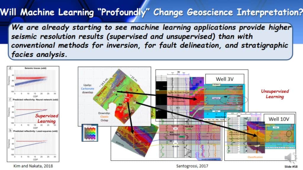
We are already starting to see machine learning applications provide higher seismic resolution results, whether supervised or unsupervised, than with inversion, fault detection, and stratigraphic facies analysis.
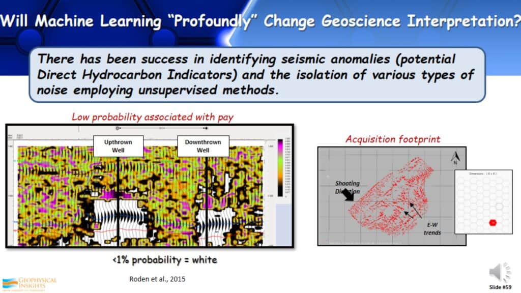
We are starting to see the identification of seismic anomalies, like previously seen with the Direct Hydrocarbon Indicators. We are also seeing the isolation of various types of noise in the data, trying to identify what is real and what is not.
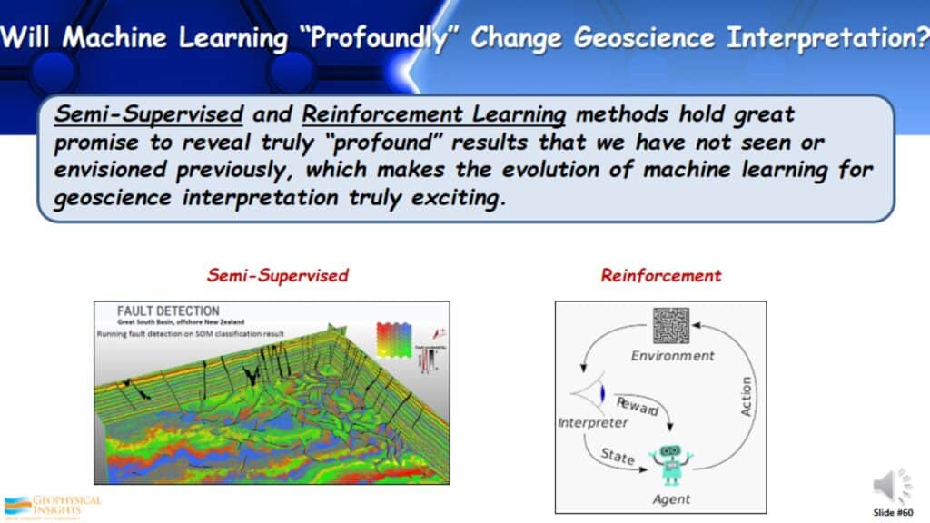
As previously stated, Semi-Supervised and Reinforcement Learning methods hold great promise and everything is shifting toward these methods. The ability to combine the best of these different machine learning approaches, to get better answers. It’s very exciting! We are in a time that we have the tools to do this and it is a very exciting interpretation tool.
Future of Machine Learning in Geoscience Interpretation
I’d like to make a prediction, given what has been shown as it relates to what interpreters should know about machine learning.
- Machine Learning can be disruptive. It can change the way you do things and give better and more accurate answers at times.
- Artificial Intelligence and Machine Learning will not replace geoscience interpreters. In my years, I have seen many technologies evolve and each evolution we hear “This will limit the interpreter”. In reality it provides more capabilities and more tools for the interpreter to do a better job.
- However, in the next five or ten years, geoscience interpreters who do not use Machine Learning will be replaced by those who do.