A few years ago, we had geophysics and geology – two distinct that were well defined. Then, geoscience came along, and it was an amalgam of geology and geophysics. Many people started calling themselves geoscientists as opposed “geologist” or “geophysicist”. But the changes weren’t quite finished. Along came a qualifying adjective, and that has to do with unconventional resource development or unconventional exploration. We understand how to do exploration, but unconventional has to do with understanding shale and finding sweet spots, but it is a type of exploration. By joining unconventional and resource development, we broaden what we do as professionals. However, the mindset of unconventional geophysics is really closer to mining geophysics than it is conventional exploration.
A few years ago, we had geophysics and geology – two distinct that were well defined. Then, geoscience came along, and it was an amalgam of geology and geophysics. Many people started calling themselves geoscientists as opposed “geologist” or “geophysicist”. But the changes weren’t quite finished. Along came a qualifying adjective, and that has to do with unconventional resource development or unconventional exploration. We understand how to do exploration, but unconventional has to do with understanding shale and finding sweet spots, but it is a type of exploration. By joining unconventional and resource development, we broaden what we do as professionals. However, the mindset of unconventional geophysics is really closer to mining geophysics than it is conventional exploration.
So, today’s topic has to do with the “holy grail” of machine learning in seismic interpretation. We’re trying to tie this to seismic interpretation only. Even if that’s a pretty big topic, we’re going to focus on a few highlights. I can’t even summarize machine learning for seismic interpretation. It’s already too big! Nearly every company is investigating or applying machine learning these days. So, for this talk I’m just going to have to focus on this narrow topic of machine learning in seismic interpretation and hit a few highlights.
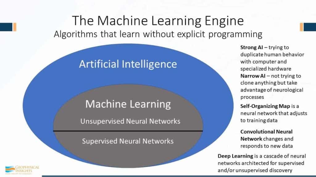
Let’s start at 50,000 feet – way up at the top. If you’ve been intimidated by this machine learning stuff, let’s define terms. Machine learning is an engine. It’s an algorithm that learns without explicit programming. That’s really fundamental. What does that mean? That means an algorithm that’s going to learn from the data. So, that means given one set of data, it’s going to come up with an answer, but with a different set of data, it will come up with a different answer. The whole field of artificial intelligence is broken up into strong AI and Narrow AI. Strong AI is coming up with a robot that looks and behaves like a person. Narrow AI attempts to duplicate the brain’s neurological processes that have been perfected over millions of years of biological development. A Self-organizing map, or SOM, is a type of neural network that adjusts to training data. However, it makes no assumptions about the characteristics of the data. So, if you look at the whole field of artificial intelligence, and then we look at machine learning as a subset of that, there are two parts: unsupervised neural networks and supervised neural networks. Unsupervised is where you feed it the data and say “you go figure it out.” In supervised neural networks, you give it both the data and the right answer. Some examples of supervised neural networks would be convolutional neural networks and deep learning algorithms. Convolutional is a more classical type of a supervised neural network, where for every data sample, we know the answer. So, a data sample might be ‘we have x, y, and z properties, and by the way, we know what the classification is a pri·o·ri. A classical example of a supervised neural network would be this: Your uncle just passed away and gave you the canning operations in Cordova, Alaska. You go to the plant to see what you’ve inherited. Let’s say you’ve got all these people standing at a beltline manually sorting fish, and they’ve got buckets eels, and buckets for flounder, etc. Being a great geoscientists, you recognize this as an opportunity to apply machine learning to possibly re-assign those people to more productive tasks. As the fish come along, you weight them, you take a picture of them, you see what the scales are, general texture, you get some idea about the general shape of them. You see what I’ve described are three properties, or attributes. Perhaps you add more attributes and are up to four or five. Now, we have 5 attributes that define each type of fish, so in mathematical terms, we’re now dealing with a five dimensional problem. We call this ‘Attribute Space’. Pretty soon, you run through all the eels and you get measurements for each eel. So, you get the neural network trained on eels. And then you run through all the flounder. And guess what – there’s going to be variations, of course, but in attribute space, of those four or five measurements that we made for each one of type of fish are going to wind up in a different cluster in Attribute Space. And that’s how we tell the difference between eels and flounder. Or whatever else you got. And everything else that you can’t classify very well, goes into a bucket that is labeled ‘unclassified’. (More on this later in the presentation.) And, you put that into your algorithm. So that’s basically the difference between supervised neural networks and unsupervised neural networks. Deep learning is a category of neural networks that can operate in both supervised and unsupervised discovery.
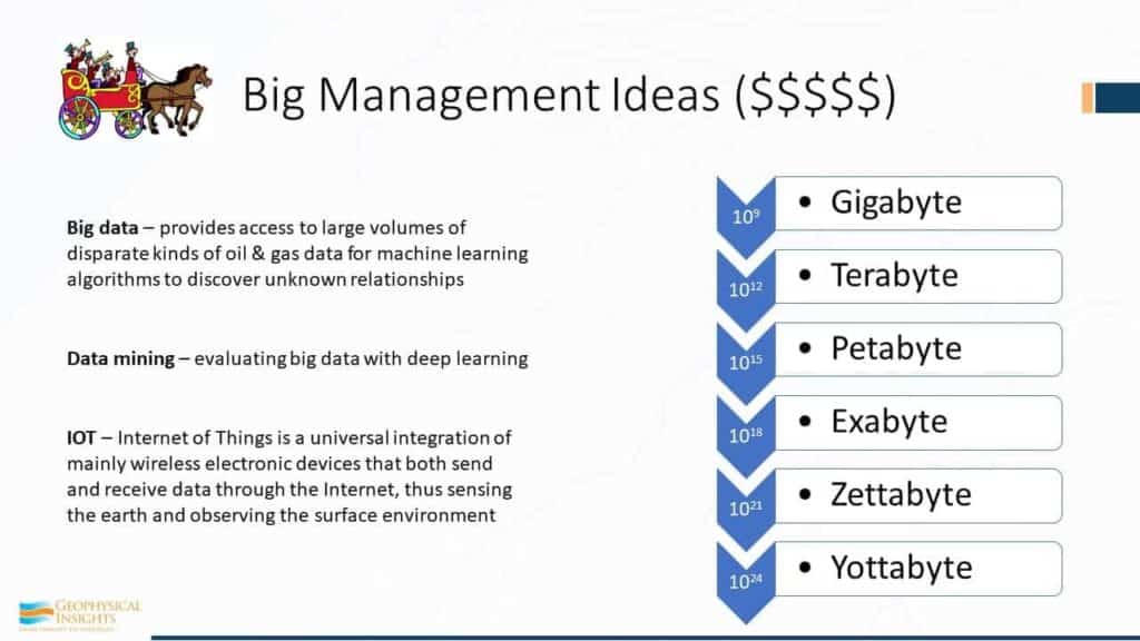
Now, before we get deeper into our subject today, I’d like to draw your attention to some of the terms: the concept of Big Data. If you remember a few years ago, if you wanted to survive in the oil and gas business, finding large fields was the objective. Well, we have another big thing today – Big Data. Our industry is looking at ways to apply the concepts of Big Data analytics. We hear senior management of E&P companies talking about Big Data and launching Data Analytics teams. So, what is Big Data or Data Analytics? It’s access to large volumes of disparate kinds of oil and gas data that is analyzed by machine learning algorithms to discover unknown relationships, those that were not identified previously. The other key point about Big Data is that it is disparate kinds. So the fact is you say “I’m doing Big Data analytics with my seismic data” – that’s not really an appropriate choice of terms. If you say “I’m going to throw in all my seismic data, along with associated wells, and my production data” – now you’re starting to talk about real Big Data operations. And, the opportunities are huge. Finally, there’s IoT – Internet of Things – which you’ve probably heard or read. I predict that IoT will have a larger impact on our industry than machine learning, however, the two are related. And why is that? Almost EVERYTHING we use can be wired to the internet. In seismic acquisition, for instance, we’re looking at smart geophones being hooked up that sense the direction of the boat and can send and receive data. In fact, when the geophones get planted, they have a GPS in each one of those things so that when it’s pulled up and thrown in the back of a pickup truck, the geophones can report their location in real-time. There are countless other examples of how IoT will change our industry.
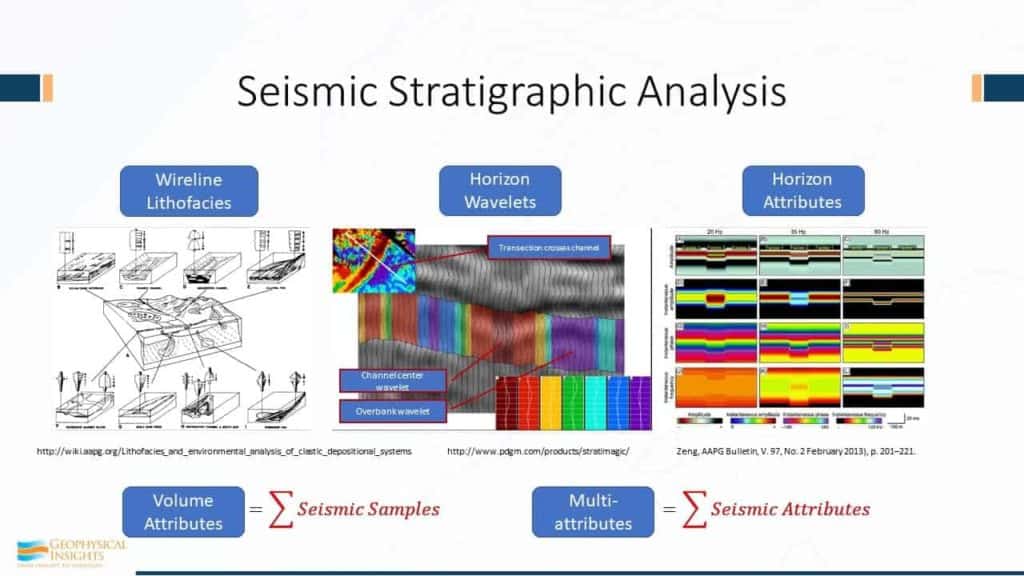
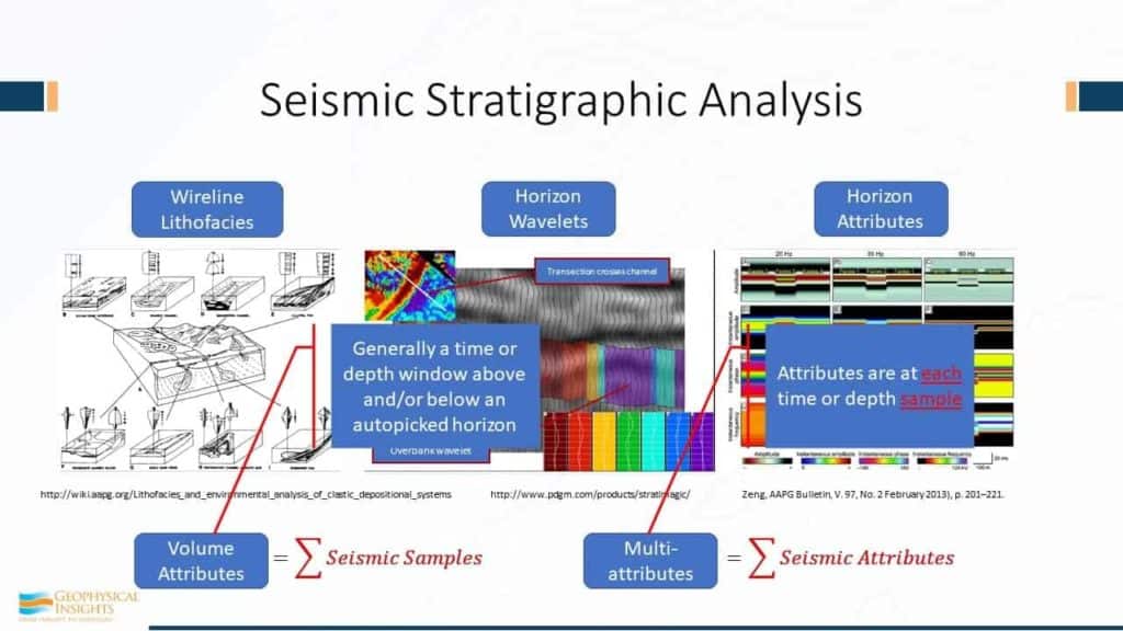
Let’s consider wirelines as a starting point of interpretation and figuring out the deposition of the environment using wireline classifications. If we pick a horizon, and based on that auto-picked horizon, we have a wavelet at every bin. We pull that wavelet out. In this auto-picked horizon, we may have a million samples and we have a million wavelets because we have a wavelet for each sample. (Some early neural learning tools were based on this concept of classifying wavelets.) Using these different classes, machine learning analyzes and trains on those million wavelets, finding say seven most significantly different. And the we go back and classify all of them. And so we have this cut shown here, across the channel and the wavelet, closest to the center, discovered to be tied to that channel. So there’s the channel wavelet, and now we have overbank wavelets, some splay wavelets – several different wavelets. And from this, a nice colormap can be produced indicating the type of wavelet.
Horizon attributes look at the properties of the wavelet along the vicinity of the horizon, at say frequency of 25 to 80 hertz with attributes like instantaneous phase. So we know have a collection of information about that pic using horizon attributes. Using volume attributes, we’ll look at a pair of horizons and integrate the seismic attributes between the horizons. This will result in a number, such as the average amplitude or average envelope value, that represents a sum of seismic samples in a time or depth interval. However, when considering machine learning, the method of analysis is fundamentally different. We have one seismic sample and associated with that sample we have multiple seismic attributes associated with that sample. This produces a multi-attribute sample vector that is the subject of the machine learning process.
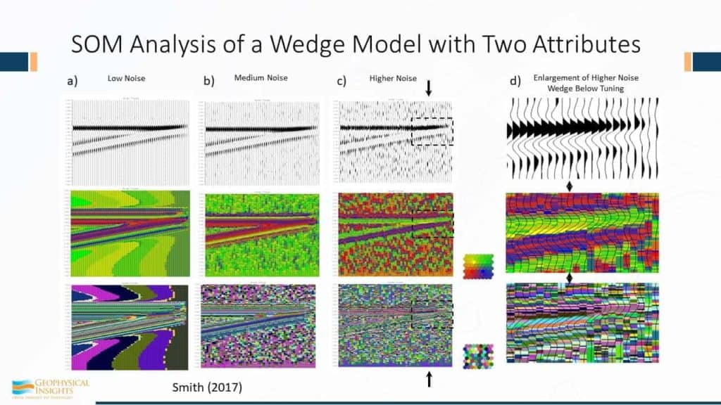
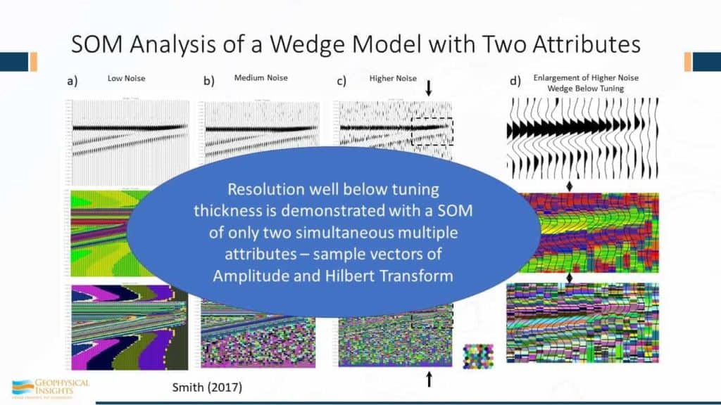
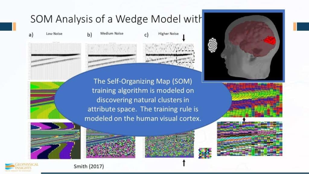
Ok, so let’s take a look at some of the results: This is a self-organizing map, analysis of a wedge using only 2 attributes. We’ve got three cases – low, medium, and high levels of noise, and in the box over here you can see tuning thickness is right here, and everything to the right of that arrow is below tuning. Now, the SOM is multi-attribute samples. And in this case, we are keeping things very simple since we only have two attributes. If you have only two attributes, you can plot them on a piece of paper – x axis, y axis. However, the classification process works just fine for two dimensions or twenty dimensions. It’s a machine learning algorithm. In two dimensions, we can look at it and decide “did it do a good job or did it not?” For this example, we’ve used the amplitude and the Hilbert Transform because we know they’re orthogonal to each other. We can plot those as individual points on paper. Every sample is a point on that scatter plot. However, if we put it through a SOM analysis, the first stage is SOM training, which is trying to locate natural clusters in attribute space, and then the second phase is once those neurons have gone through the training process, we then take the results out and classify ALL the samples. So, we have here the results – every single sample is classified. Low noise, medium noise, high noise, and here are the results here. If you go to tuning thickness, we are tracking with SOM analysis events way below tuning thickness. And the fact that there’s the top of the wedge or … this one right here is where things get below tuning thickness. Eventually tip the corresponding trace right over there. Now, there’s a certain bias. We are using here for this analysis a two-dimensional topology – it’s two dimensions, but also the connectivity is hexagonal connectivity between these neurons, which is made use of during the training process. And there’s a certain bias here because this is a smooth colormap. By the way, these are colormaps as opposed to colorbars. Right? Color maps, not colorbars. In terms of color MAPS, you can have four points of connectivity, and then it’s just like a grid. Or 6 points of connectivity, and then it’s hexagonal. That helps us understand the training that was used. Well, there’s a certain bias about having smooth colors and we have attempted in this process here – there’s 8 rows and 8 columns – every single one of those has gone looking for a natural cluster in attribute space. Although it’s only two dimensions, they are still is a hunting process. Each of these 64 neurons, after the training process, are trying to zero in on a natural cluster. And there’s a certain bias here in using smooth colors because that happens like yellow and greens and here’s blues and reds. Here’s a random color – and you can see the results. But even if we use random colors, we are still tracking events way below tuning thickness using the SOM classification.
We are demonstrating the resolution well below tuning. There’s no magic. We use only two attributes – the real part and the imaginary part, which is the Hilbert Transform, and we are demonstrating the SOM characteristics of training using only two attributes.
The self-organizing map, SOM, training algorithm is modeled on discovering of natural clusters in attribute space, using training rules based upon the human visual cortex. Conceptually, this is a simple but powerful idea. We can see examples in nature of simple rules that lead to profound results.
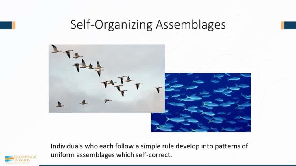
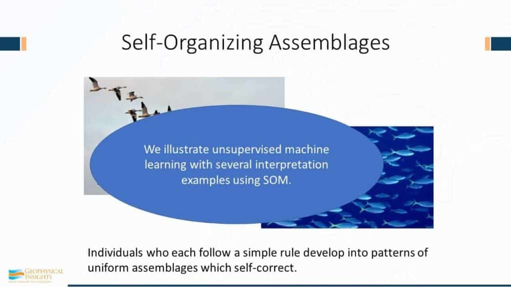
So, the whole idea behind self-organizing assemblages is the following: Snow geese and fish are both examples of self-organizing assemblages. Individuals follow a simple rule. The individual goose is just basically following a very simple rule: Follow the goose in front of me, just a few feet behind and either left or right. It’s a simple as that. That’s an example of self-organizing assemblage, but yet some of the properties of that are pretty profound, because once they get up to altitude, they can go for a long time and long distances using the slipstream properties of that “v” formation. The basic rule for a schooling fish is ‘swim close to your buddies. Not so close that you’ll bump into them, and not so far away that it doesn’t get represented as a school of fish.’ When the shark swims by, the school needs to look like one big fish. If those individual fish were too far apart, the shark would see the smaller isolated fish as easy prey. So, there’s even a simple rule here of a optimum distance one to the other. These are just two examples of where simple rules produce complex results when applied at scale.
Unsupervised neural networks work, which classify the data, also work on simple rules but operating on large volumes of seismic samples in attribute space.
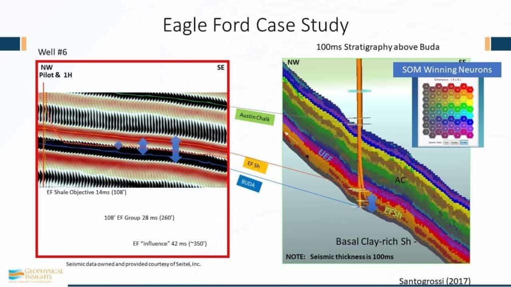
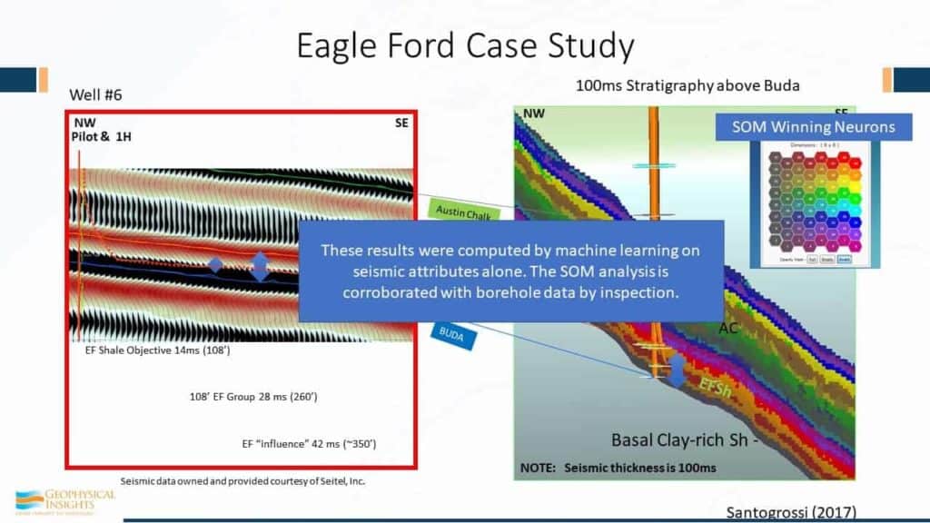
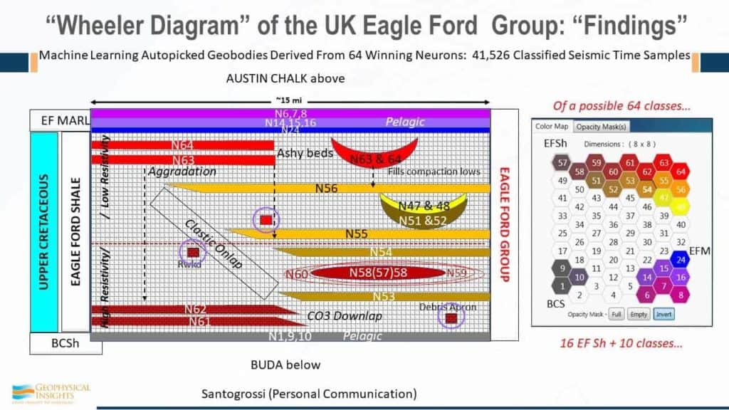
The first example is the Eagle Ford case study. Patricia Santagrossi published these results last year. This is a 3D survey of a little over 200 square miles. The SOM analysis was run between the Buda and the Austin Chalk and the Eagle Ford is right above the Buda in this little region right there. The Eagle Ford shale layer was 108′ thick, which is only 14 ms. Now both the Buda and Austin Chalk are known , strong peak events. So, if you count how many cycles we go through here, peak trough, kind of a doublet, trough, peak. The good stuff here is basically all the bed from one peak to one trough. Conventional seismic data. Here’s the Eagle Ford shale as measured right at the Buda break well there. We have both a horizontal and a vertical well right here. And that trough is associated with the Eagle Ford Shale. That trough and that peak. So, this is the SOM result with an 8×8 set of neurons that are used for the training. Look at the visible amount of detail here. Not just between the Buda and the Austin Chalk, but actually you can see how things are changing, even along the formation here, within the run of the horizontal well. Because every change in color here corresponds to a change in neuron.
These results were computed by machine learning using seismic attributes alone. We did not tie the results to any of the wells. The SOM analysis was run on seismic samples with multiple attributes values. The key idea here is simultaneous multi-attribute analysis using machine learning. Now, let’s look further at this Eagle Ford case study.
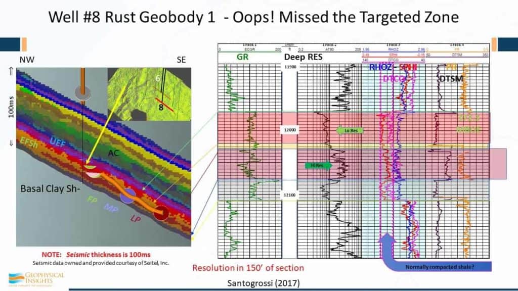
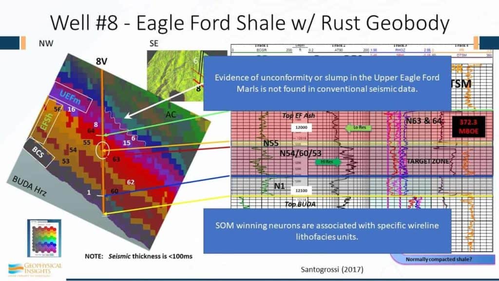
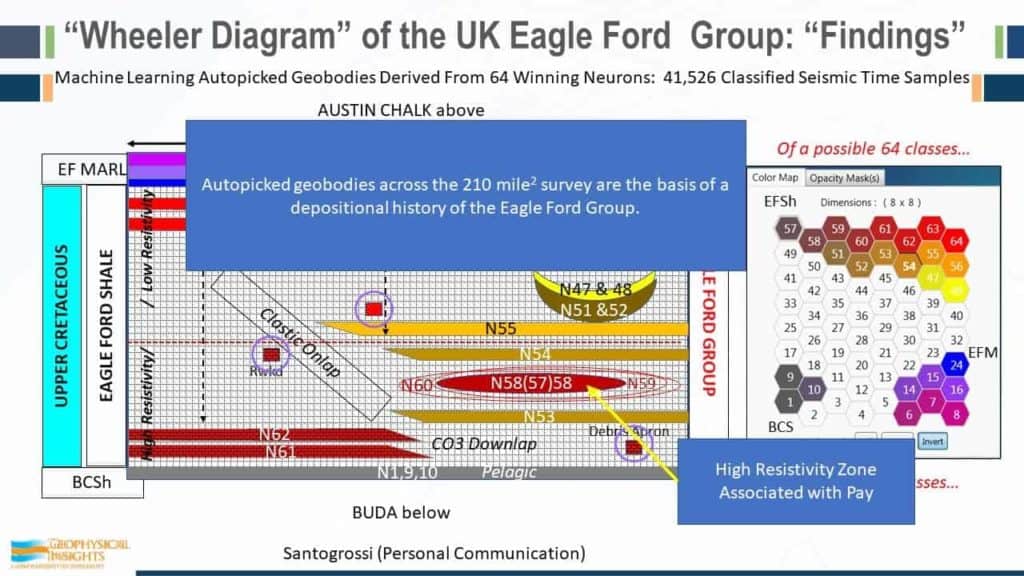
These are results computed by machine learning using seismic attributes. We did not skew the results and tie them to any of the wells. They were not forced to fit the wells or anything else. The SOM analysis was run strictly on seismic data and the multi-attribute seismic samples. Again , the right term is simultaneous multi-attribute analysis. Multi-attribute, meaning it’s a vector. In our analysis every single sample is being used simultaneously to classify the data – a solution. So although this area is 200 square miles from an aerial view, between the Buda and the Austin Chalk, we’re looking at every single sample – not just wavelets. By simple inspection, we can see that the results corroborate the results of applying machine learning with the well logs, but there has been no force fitting of the data. These arrows are referring to the SOM winning neurons. If we look at detail, here is Well #8, a vertical well in the Eagle Ford shale. The high resistivity zone is right in here. That could be tied into the red stuff. So, here again we’re dealing with seismic data on a sample-by-sample basis.
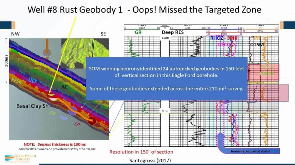
The SOM winning neurons identified 24 geobodies, autopicked in 150 feet of vertical section at this well on #8 in the Eagle Ford borehole. Some of the geobodies – not all of them – some of them track the underwells and went over the entire 200 sq. mile 3D survey.
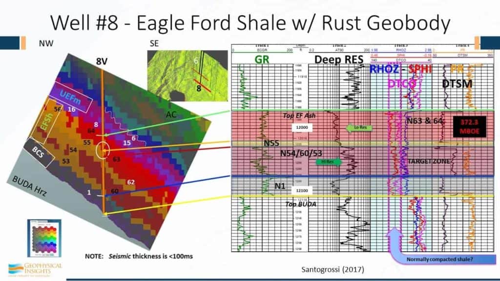
This is to zero in a little bit more . So I can give you some association here. This is the high resistivity zone is correlating with winning neuron 54, 60, and 53 in this zone right in here. There’s the Eagle Ford Ash that is identified with neurons 63 and 64. And Patricia even found to tie in with this marker right here – this is neuron 55.
And this well, by the way, well #8, was 372 Mboe. SOM classification neurons are associated with specific wireline lithofacies units. That’s really hard to argue against. We have evidence, in this case up here for example, of an unconformity where we lost a neuron right through here and then we picked it up again over there. And, there is evidence in the Marl of slumping of some kind. So, we’re starting to understand what’s happening geologically using machine learning. We’re seeing finer detail – more than we would have using conventional seismic data and single attributes.
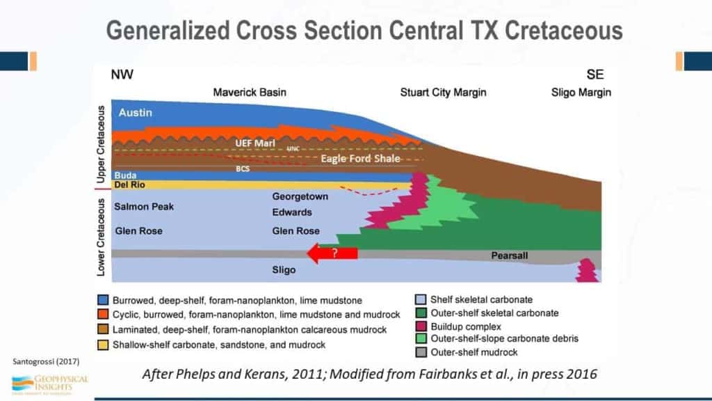
Tricia found a generalized cross section of Cretaceous in Texas, northwest / southeast towards the gulf. Eagle Ford shale fits in here below the Marl and there’s an unconformity between those two – she was able to see some evidence of that.
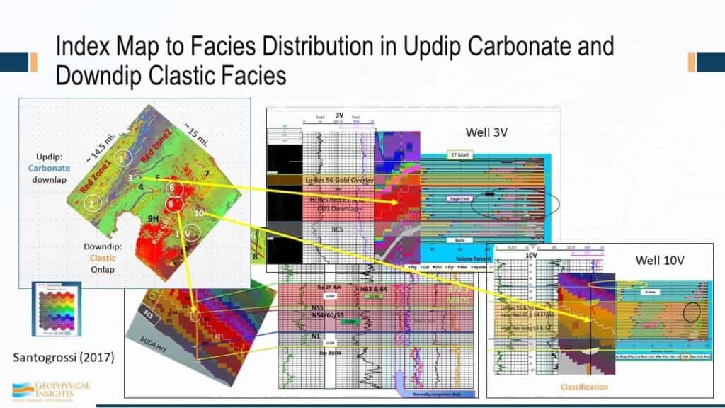
The well that we just looked at was well #8, and it ties in with the winning neuron. Let’s take a look at another well, say for example, well #3, a vertical well with some x-ray diffraction associated with it. We can truly nail this stuff with the real lithology, so not only do we have a wireline result, but we also have X-ray diffraction results to corroborate the classification results.
So, of the 64 neurons, over 41,000 were classified as “the good stuff”.. Not on a sample basis, so you can integrate that – you can tally all that stuff up and start to come up with estimates.
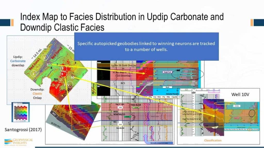
So, specific geobodies relate to winning neuron that we’re tracking – #12 – that’s the bottom line. And from that we were able to develop a whole Wheeler diagram for the Eagle Ford group for the survey. And the good stuff are the winning neurons 58 and 57. They end up on the neuron topology map here, so those two were associated with the wireline lithofacies footstep – the high resistivity part of the Eagle Ford shale. But she was able to work out additional things, such as more clastics and carbonates in the west and clastics in the southeast. And, she was able to work out not only Debris Apron, but the ashy beds and how they tie in. Altogether, these were the neurons associated with the Eagle Ford shale. These were the neurons – 1, 9, and 10, that’s the basal clay shale. And the Marls were associated with these neurons.
So, the autopicked geobodies, across the survey on the basis we’re developing the depositional environment of the Eagle Ford that compare favorable with the well logs. Using seismic data alone, one of our associates received feedback to the effect that “seismic is only good in conventionals, just for the big structural picture.” Man, what a sad conclusion that is. There’s a heck of a lot more out of this high resistivity zone pay that was associated with two specific neurons, demonstrating that this machine learning technology is equally applicable to unconventionals.
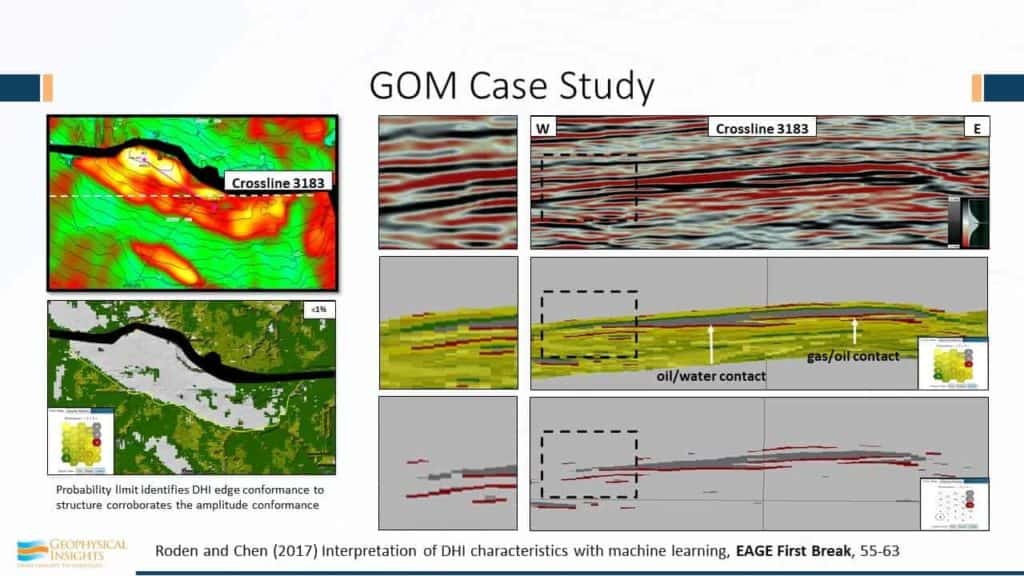
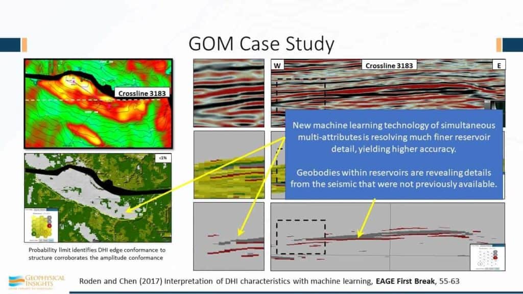
The second case study here is the Gulf of Mexico, by my distinguished associate, Mr. Rocky Roden. This is not deepwater – only approximately 300 feet. Here’s a north fault amplitude buildup. Here, these are time contours and the amplitude conformance to structure is pretty good. In this crossline – 3183 – going from west to east is the distribution of the histogram of the values. You can see here in the dotted portion, this is just the amplitude display, and the box right here is a blowup of the edge right there of that reservoir. What you can see here is the SOM classification using colors. Red is associated with the gas-over-oil contact and oil-over-water contact. A single sample. So here we have the use of machine learning to help us find fluid contacts, which are very difficult to see. This is all without having bandwidth, frequency range, point source, point receivers – it isn’t a case of everything dialed in just the right way. The rest of the story is just the use of machine learning. However, it’s machine learning on not just samples of single numbers, but each sample as a combination of attributes; as a vector. Using that choice of attributes, we’re able to identify fluid contacts. For easier viewing, we make all these others transparent and only show those that you can see visually here of what has been estimated using the classifier of the fluid contacts and also the hills. In addition, look at the edges. The ability to define the edge of the reservoirs and come up with volumetrics, is pretty clear to be superior. Over here on the left, Rocky’s taken the “goodness of fit”, which is an estimate of the probability of how well each of these samples fits the winning neuron, and by lowering the probability limit, and saying “I just want to look at the anomalies”, that edge of the amplitude conformance of structure, I think is clearly better than what you would have using amplitude alone.
So, new machine learning technology stuff using simultaneous multi-attributes is resolving much finer reservoir detail than we’ve had in the past, and the geobodies that fit the reservoirs are revealed in the details, frankly, previously not available.
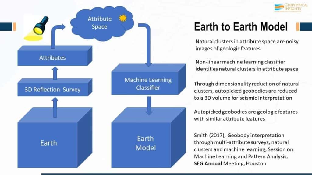
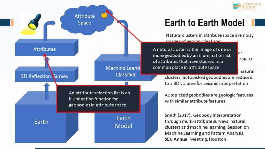
In general, this is what our “Earth to Earth” model looks like. If we start here with the 3D survey, and then from the 3D survey, we decide on a set of attributes. We take all our samples, which are vectors because of our choice of attributes, and then literally, plot them in attribute space. If you’ve 5 attributes, it’s 5-dimensional space. If you have 8 attributes, it’s 8-dimensional space. And your choice of attributes is going to illuminate different properties of the reservoir. So, the choice of attributes that Rocky used helped to zero in on those fluid contacts, would not be the ones he would use to illuminate the volume properties or the absorption properties, for example. Once the attribute volumes is in attribute space, we use a machine learning classifier to analyze and look for natural clusters of information in attribute space. Once those are classified in attribute space, the results then, are presented back in a virtual model, if you will, of the earth itself. So, our job here is our picking geobodies, some of which have geologic significance and some of which don’t. The real power is in the natural clusters of information in attribute space. If you have a channel and you’ve got the attributes selected to illuminate channel properties, then, every single point that is associated with the channel, no matter where it is, is going to concentrate in the same place in attribute space. Natural clusters of information in attribute space are all stacking. The neurons are hunting, looking for natural clusters, or higher density, in attribute space. They do this using very simple rules. The mathematics behind this process were published by us in the November 2015 edition of the Interpretation journal, so if you would like to dig into the details, I invite you to read that paper, which is available on our website.
Two keys are: 1. Attribute selection list. Think about your choice of attributes as an illumination function. What you are trying to do with your choice of attributes is an illumination function of the real geobodies in the earth and how they end up as natural clusters in attribute space. And that’s the key. 2. Neurons search for clusters of information in attribute space. Remember the movie, The Matrix? The humans had to be still and hide from the machines that went crazy and hunted them. That’s not too unlike what’s going on in attribute space. It’s like The Matrix because the data samples themselves don’t move. They’re just waiting there. It’s the neurons that are running around in attribute space, looking for clusters of information. The natural cluster is an image of one or more geobodies in the earth, but it’s been illuminated in attribute space, totally depending on the illumination list. It stacks in common place in attributes – that’s the key.
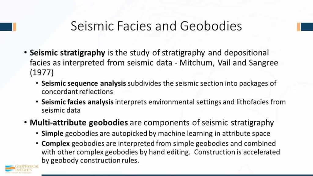
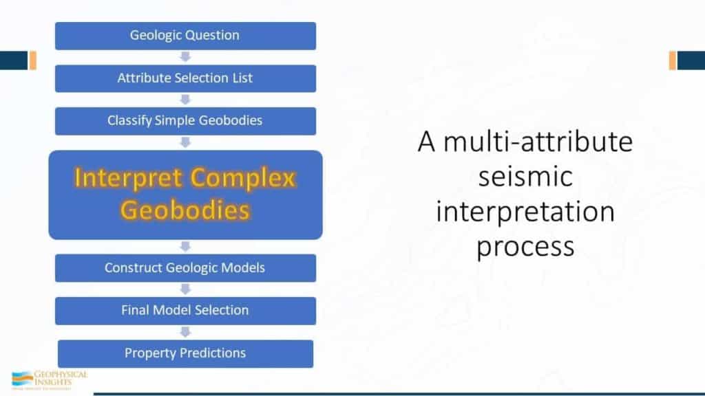
Seismic stratigraphy is broken up into two levels here: first is seismic sequence analysis where you look at your seismic data and you organize it and break it up in to packets of concordant reflections. It’s pretty straightforward stuff – chaotic depositional patterns. And then after you have developed a sequence analysis, you can categorize the different sequences. You have a facies analysis trying to infer the depositional setting. Is the sea level rising? Is it falling? Is it stationary? All this naturally falls in because the seismic reflections are revealing geology on a very broad basis. Well, the attribute – it’s hunting geobodies as well. Multi-attribute geobodies are also components of seismic stratigraphy. We define it this way: a simple geobody has been auto-picked by machine learning in attribute space. That’s all it is – we’re defining a simple geobody. We all know how to run an auto-picker. In 15 minutes, you can be taught how to run an auto-picker in attribute space. Complex geobodies are interpreted by you and I. We look at the simple geobodies and we composite those just the way we saw in that wheeler diagram. We combine those to make complex geobodies. We give it a name, some kind of texture, some kind of surface – all those things are interpreted geobodies and the construction of these complex geobodies can be sped up by some geologic rule-making.
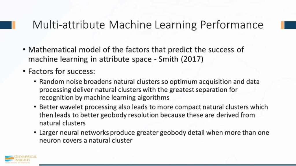
Now the mathematical foundation we published in 2015 ties this altogether pretty nicely. You see, machine learning isn’t magic. It depends on the noise level of the seismic data. Random noise broadens natural clusters in attribute space. What that means then, is that we’re attenuating noise so optimum acquisition and data processing, delivering natural clusters with the greatest separation. In other words, nice, tight clusters in attribute space will be much easier for the machine learning algorithm to identify when you have nice, clean identification and separation. So, acquisition and data processing matters. However, this isn’t talking about coherent noise. Coherent noise is something else. Because with coherent noise, you may have an acquisition footprint, but that forms a cluster in attribute space and one of those neurons is going to go after that just as well because it’s an increase in information density in attribute space and voila – you have a handful of neurons that are associated with an acquisition footprint. Coherent noise can be deducted by the classification process where the processor has merged two surveys. Second thing: Better wavelet processing leads to narrower, natural clusters, more compact natural clusters leads to better geobody resolution because geobodies are derived from natural clusters. Last but not least, larger neural networks produce greater geobody details. You run a 6×6, an 8×8 and a 10×10 2D Colormaps, you eventually get to the point where you’re just swamped with details and you just can’t figure this thing out. We see that again and again. So, it’s better to look at the situation from 40K feet, and then 20, and then 10. Usually, we just go ahead and run all three SOM runs all at once to get them all done and to examine them in increasing levels of detail.
I’d like to now switch gears on something entirely different. Put the SOM box here aside for a minute, and let’s revisit the work Rocky Roden did in the Gulf of Mexico . Rocky came up with an important way of thinking about the application of this new tool.
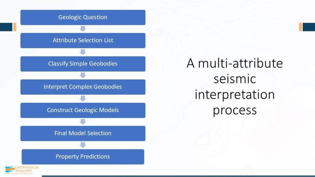
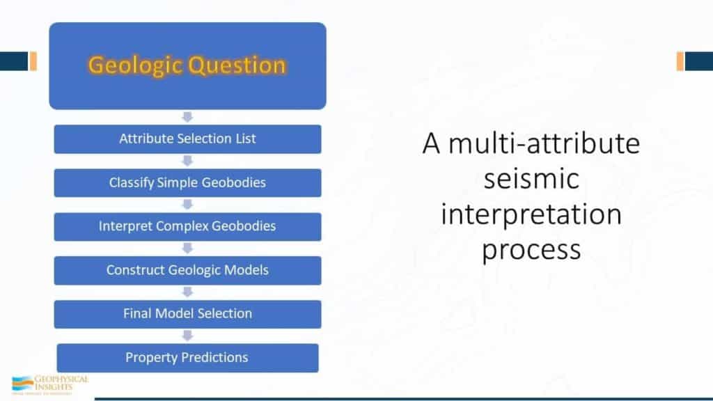
In terms of using multi-attribute seismic interpretation – think of it as a process and what’s really important is starting with the geologic question of what you want to answer. For example: we’re trying to illuminate channels. Ok, so there are a certain set of attributes that would be good. So, what we have then here is, ask the question first. Firmly have that in your mind for this multi-attribute seismic interpretation process.
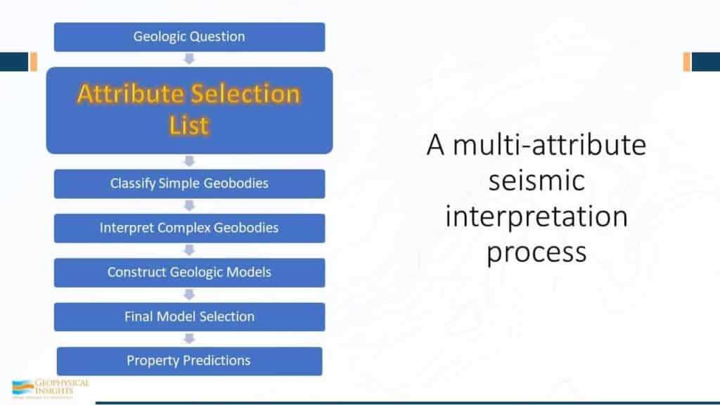
There’s a certain set of attributes for the geologic question, and the terminology for that set is the “attribute selection list”. When you do an interpretation like this, you really need to be aware of the current attributes being used when looking at the data. Depending on the question, we then take the discipline and we say “well, if this is the question you’re asking”, this attribute selection list is appropriate. Remember, the attribute selection list is an illumination function.
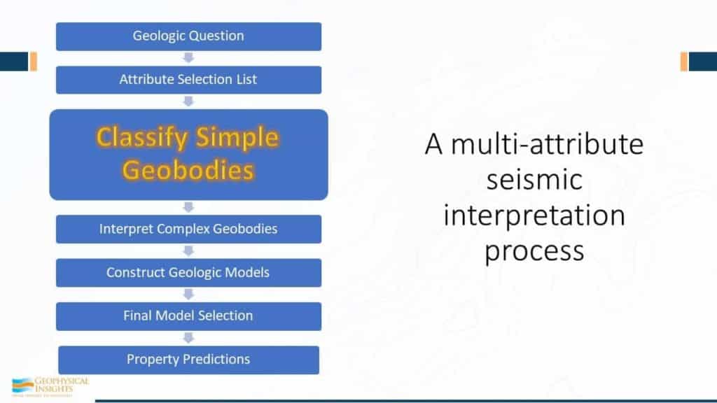
Once you have the geologic process, the next step is the attribute selection list, and then classify simple geobodies, which is auto-picking your data in attribute space and looking at the results.
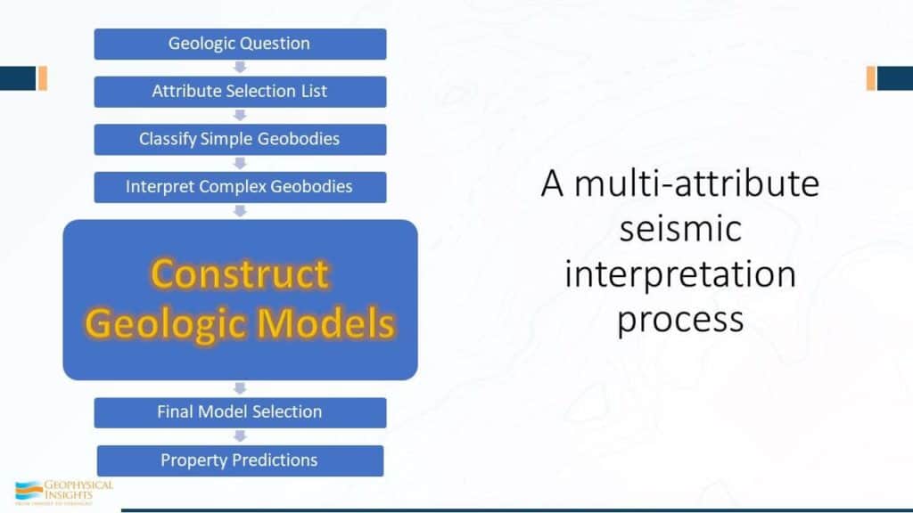
Now, this just doesn’t happen in back and it just doesn’t happen at once – it’s an iterative process. So, interpreting complex geobodies is basically more than one SOM run, and more than one geologic question. And interpreting these results at different levels – how many neurons, that sort of thing, this is a whole seismic interpretation process. Interpreting these complex geobodies is the next step.
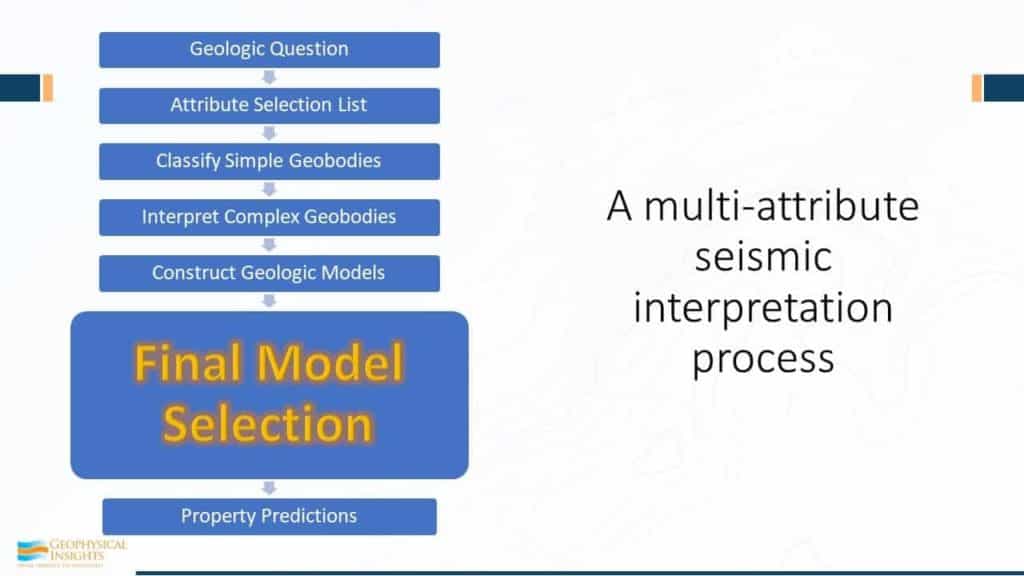
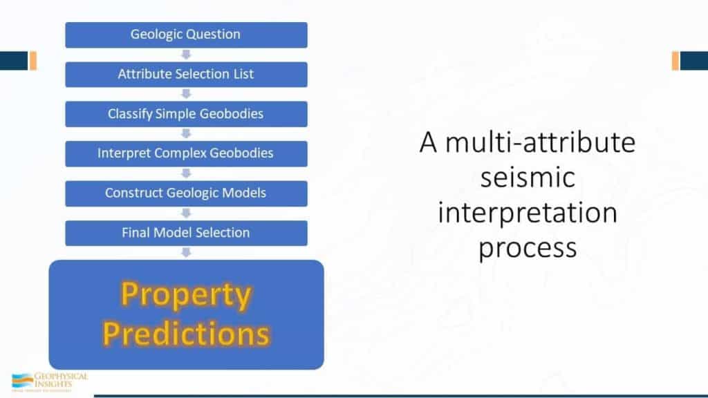
We’re looking at results and constructing geologic models. Decide which is the final geologic model, and then our last step is making property predictions.
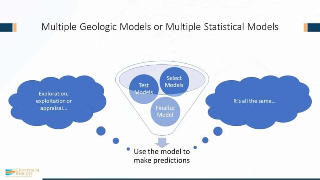
So, in the world of multiple geologic models, or multiple statistic models, it really doesn’t make any difference. We select the model, we test the model, we select a bunch of models, we test those models, and we choose one! Why? Because we want to make some predictions. There’s got to be one final model that we decide on as professional that this is most reliable and we’re going to use it. Whether it’s exploration, exploitation, or even appraisal, same methodology – it’s all the same for geologic models and statistical models.
The point here boils down to something pretty fundamental. As exploration geophysicists, we’re in the business of prediction. That’s our business. The boss wants to know “where do you want to drill, and how deep? And what should we expect on the way down? Do we have any surprises here?” They want answers! And we’re in the business of prediction.
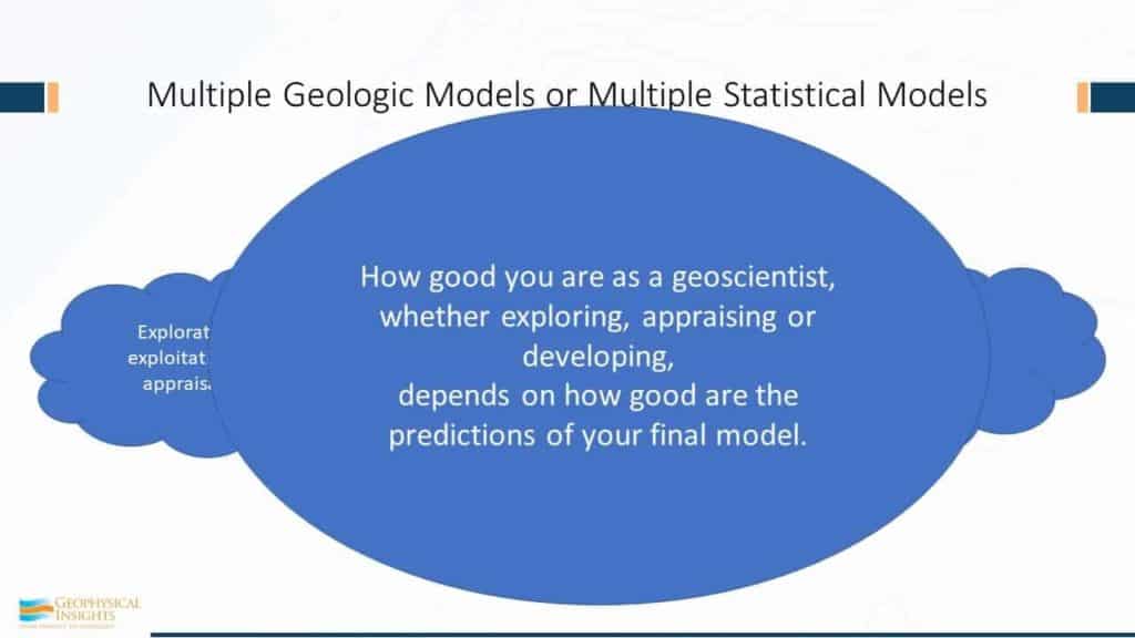
So how good you are as a geoscientist depends, fundamentally, on how good are your predictions of your final model? That’s what we do. Whether you want to think about it like that or not, that’s really the bottom line.
So how good you are as a geoscientist depends, fundamentally, on how good are your predictions of your final model? That’s what we do. Whether you want to think about it like that or not, that’s really the bottom line.
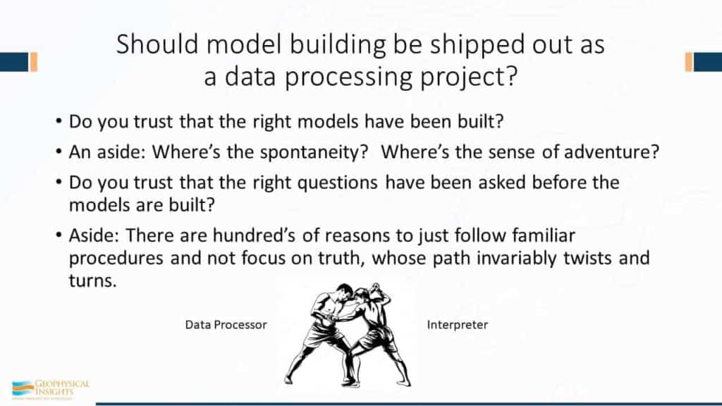
So this is really about model building for multi-attribute interpretation – that’s the first step. Then we’re going to test the model and choose the model. Ok, so, should that model-building be shipped out as a data processing project? Or through our geo-processing people? Or is that really something that should be part of interpretation? Do you really trust that the right models have been built from geoprocessing? Maybe. Maybe not. If it takes 3 months, you sure hope you have the right model from a data processing company. And foolish, foolish, foolish if you think there’s only one run. That’s really dangerous. That’s a kiss and a prayer, and oh, after three months, this is what you’re going to build your model on. So, as an aside, if you decide that building models is a data processing job, where’s the spontaneity? And I ask you – where’s the sense of adventure? Where’s the sense of the hunt? That’s what interpretation is all about – the hunt. Do you trust that the right questions have been asked before the models are built? And my final point here is that there are hundred’s of reasons just to follow procedure. Stay on the path and follow procedure. Unfortunately, nobody wants to argue. The truth here is what we’re looking for. And truth, invariably – that path has twists and turns. That’s exploration. That’s what we’re doing here. That’s fun stuff. That’s what keeps our juices going… about finding those little twists and turns and zeroing in on finding truth.
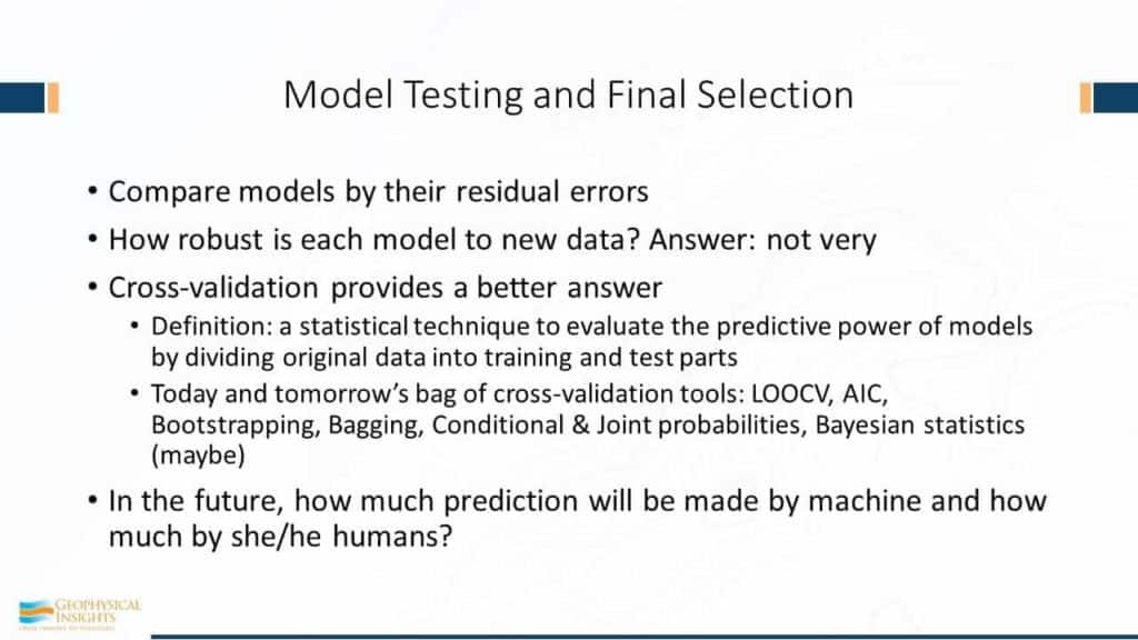
Now model testing and final selection have begun when models are built and you decide which is the right one. For example, you generate 3 SOMs – an 8×8, 12×12, 4×4, and you look at results and the boss says “ok, you’ve been monkeying around long enough, what’s the answer? Give me the answer”… “Well…hmm…” you respond. “I like this one. I think 8×8 is the right one.” Now, you could do that, but you might not want to admit it to the boss! One quantitative way of comparing models would be to look at your residual errors. The only trouble with that is it’s not very robust. However, a quantitative assessment – comparing models – is a good way to go. So, there is a better methodology – better than just comparing residual errors – this is a whole field of cross-validation methodologies. Not going to go into that stuff right here, but some cross-validation tools: bootstrapping, bagging, and even Bayesian statistics are helpful tools in helping us prepare models and helping us figure out the model that is robust and in the face of new data is going to give us a good strong answer – NOT the answer that fits the data the best. Think about the old problem of fitting a least squares line through some data. You write your algorithm in python or whatever tool, and it kind of fits through the data, and the boss goes “I don’t know why you’re monkeying around with lines. I think this is an exponential curve because this is production data.” So, you make an exponential curve. Now, this business of cross-validation, think about this: fitting a polynomial to the data: two terms, a line, three terms, a parabola, four terms … until n… we could make n equal 15 and by golly there’s no possibility of error – we crank that thing down. The trouble is, we have over-fit the data. It fits this data perfect, but some new data comes in and it’s a terrible model because the errors are going to be really high. It’s not robust. So, this whole comes up to cross validation methodology is really very important. The future here is, “who’s going to be making the prediction – you, or the machine?” I maintain to make good decisions, it’s going to be us! We’re the ones that will be making the right characteristics – because we’ll leverage machine learning.
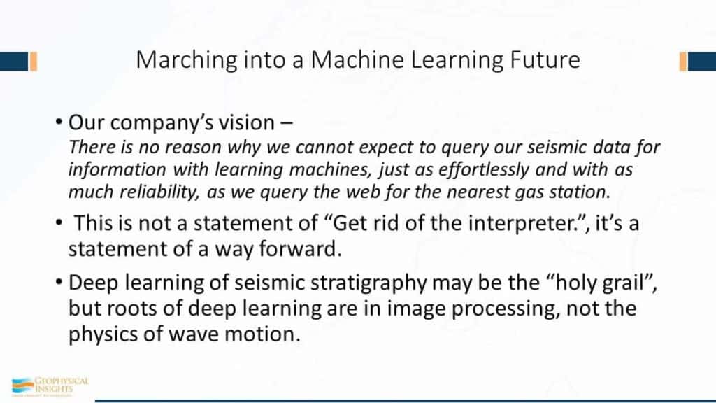
Let’s take a look at Machine Learning. Our company vision is the following: “There’s no reason why we cannot expect to query our seismic data for information with learning machines, just as effortlessly and with as much reliability as we query the web for the nearest gas station.” Now this statement of where our company is going is not a statement of “get rid of the interpreters“. It’s a statement, in my way of thinking, and in all of us at our operations, it’s a statement of a way forward. Because truly, this use of machine learning is a whole new way of doing seismic interpretation. It’s using it as a tool – it’s not replacing anybody. Deep learning, which is an important for seismic evaluation, might be a holy grail, but its roots are in image processing, not in the physics of wave motion. Be very careful with that. Image processing is very good at telling the difference between Glen and me from that have pictures of us. Or if you have kitties and you have little doggies, image processing can classify those, even right down to those that you’re not real certain whether it’s a dog or cat. So, deep learning is focused on image processing and also on the subtle distinctions between what is the essence of a dog and what is the essence of a cat, irrespective of whether the cat is laying there or standing there or climbing up a tree. That’s the real power of this sort of thing.
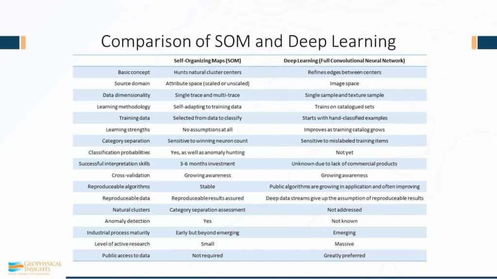
Here’s a comparison of SOM and Deep Learning in terms of all of its properties, and there’s good and bad things about each one of these. There’s no magic about any one of these. Not to say one’s better than the other. I would like to point out that unsupervised machine learning trains by discovering natural clusters in attribute space. Once those natural clusters have been identified in attribute space, attribute space is carved up and say any samples to this region right in here in attribute space corresponds to this winning neuron and over here is that winning neuron. Your data is auto-picked and put back in 3-dimensional space in a virtual 3D survey. That’s the essence of what’s available today. Supervised machine learning trains on patters that it discovers on amplitude data alone. Now there are two deep learning algorithms that are popular today. One’s called Convolutional Neural Network, which learns by visual patterns, faces, sometimes called eigenfaces, uses PCA. And then there’s fully convolutional networks, which are using sample size patches and full connections between the network layers.
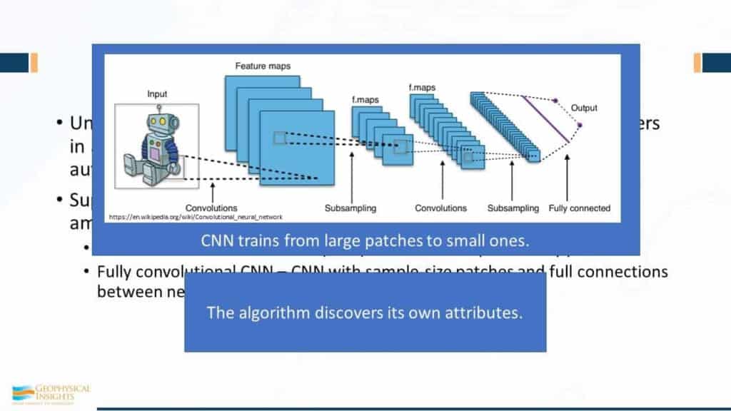
Here’s a little cartoon showing you this business about layers. This is the picture and trying to identify the little features of this, you can’t say that this is a robot, as opposed to a cat or a dog, until it goes through this analysis. Using patching and features maps, using different features for different things, it goes from one patch to the next to the next, until finally – your outputs here -well, it must be robot, dog, or kitty. It’s a classifier using the properties it has discovered in a single image. The algorithm has discovered its own attributes. You might say “that’s pretty cool”. And indeed it is, butits only using the information seen in that picture. So, it’s association – it’s the texture features of that image.
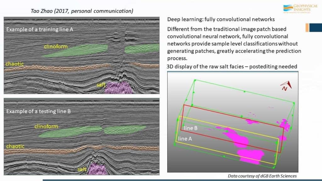
Here’s an example from one of our associates – Tao Zhao – he’s been working in the area of full convolutional networks. This example is where he’s done some training – training lines A – clinoforms here, chaotic deposition here, maybe some salt down there, and then some concordant reflections up top. Here’s an example of the results of the FCN. And then here is the classification of salt down here. So, the displays here are examples of full convolutional networks.
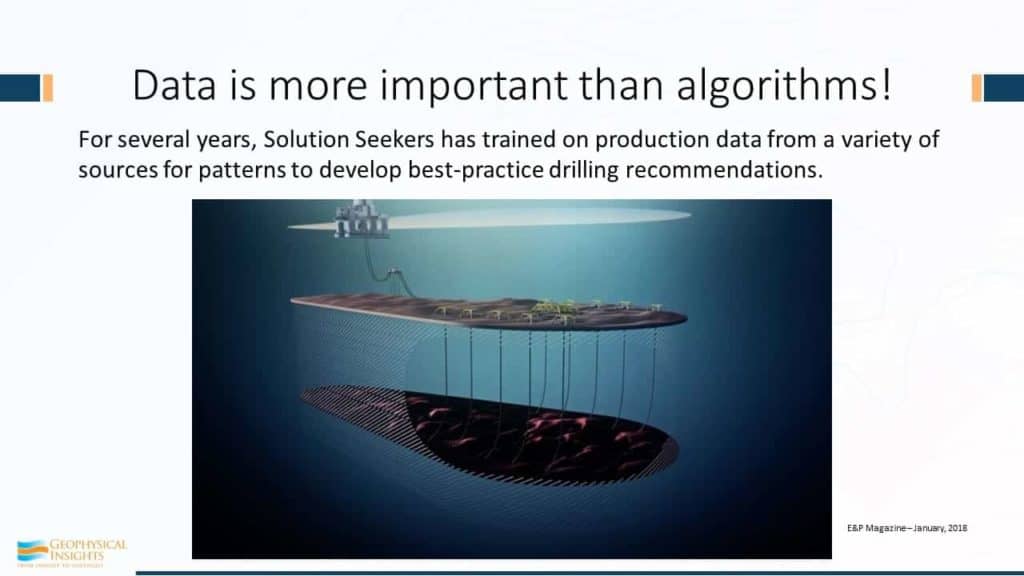
One final point and then I’ll sit down: Data is more important than the algorithms. The training rules are very simple. Remember the snow geese? Remember the fish? If you were a fish or if you were a snow goose, the rules are pretty simple. There’s a fanny – I’m gonna be about 3 feet behind it, and I’m not gonna be right behind the snow goose ahead of me – I want to be either to the left or the right. Simple rule. You’re a fish, you want to have another fish around you of a certain distance. Simple rules. What’s important here is data is more important than the algorithms. Here is an example taken from E&P Magazine this month (January). Several years this company called Solution Seekers has been training on production data using a variety of different data and looking for patterns to develop best practice drilling recommendations. Kind of a cool big-picture kind of a concept.
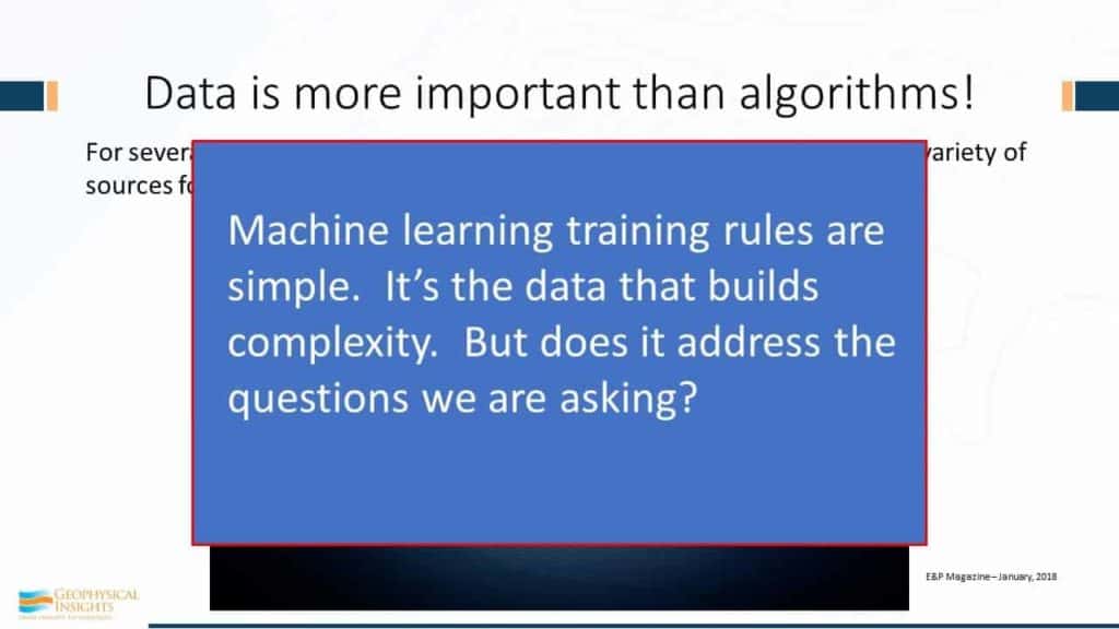
So machine learning training rules are simple – the real value is the classification of results it’s the data the builds the complexity. My question to you is: Does this really address the right questions? If it does, extremely valuable stuff. If it misses the direction of where we’re going – the geologic question – it’s not that useful.
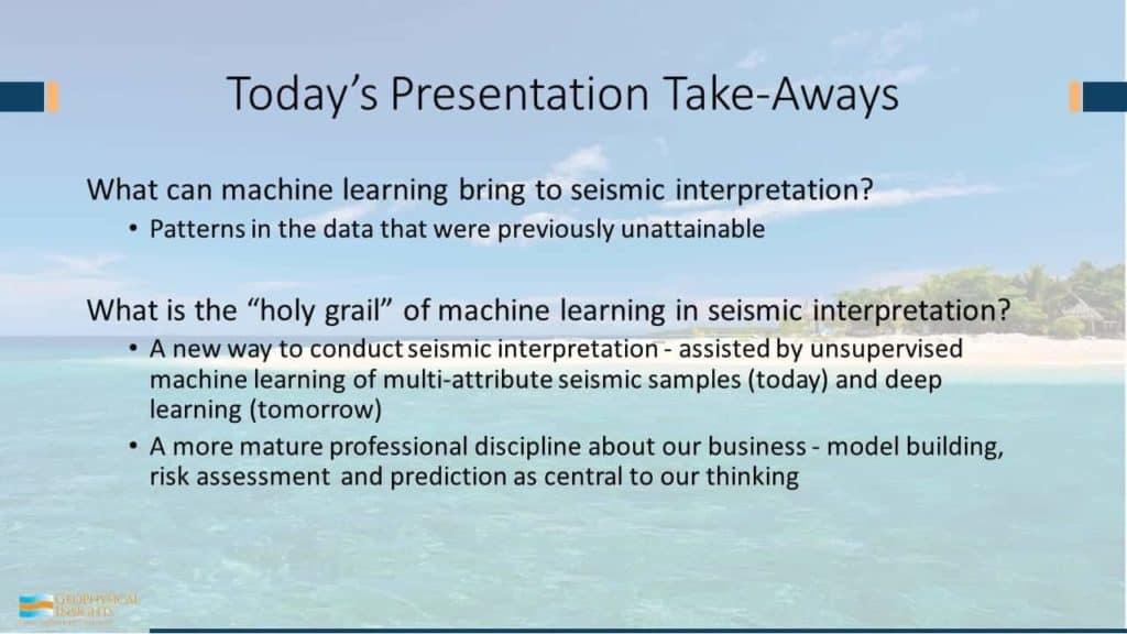
So, here are your takeaways. What does machine learning bring to seismic interpretation? It brings patterns that are previously unattainable. It’s working in an attribute space far higher than we can operate in. 3 spaces is ok… maybe we can make it to four because we can color up our points. Ok, so that’s four… but when you really get right down to it, you have a whole 3D survey, you’ve got 20 million sample points, each one is a vector… let this machine try to figure this stuff out. So, patterns are what machine learning helps us with in our seismic interpretation. And on the second thing here: the holy grail, if there is a holy grail – two things: It’s a new way to conduct seismic interpretation. This is a wave that’s on the way. I can state that with great certainty. How can I state that with great certainty? Because your boss thinks so. All the bosses have bought into this – data mining, deep learning – gotta have some of that. What is our geologist and geophysicist staff doing? Aren’t they using any of that stuff? They should be down there trying to find oil and gas and discovering relationships that they’ve never seen before. Let’s just be careful about this sort of thing because our data is fundamentally different from pictures of kitties and dogs and newborn babies. The web is filled with free data that’s already been classified. Now, we’re feeling around data where we’re just learning the properties of those natural clusters. Where we stand today, our understanding of our seismic data and multi-attributes is going to be very primitive compared to what we’ll have two years from now. We’ll have a whole lot better appreciation about what to be looking for. And supervised neural networks are going to make a whole lot more sense. So today, unsupervised machine learning of multi-attribute seismic samples is the new way of doing things – another tool to do interpretation. Tomorrow probably will be deep learning in one form or another. Second point – it’s a more professional discipline about our business, in terms of thinking about building models, assessing risk of the models, and figuring out with particular questions which is the best model, and then making predictions. This whole process of model building, then choosing a model, and then ultimately making a prediction. It leads to a much more by developing the center of what we do in our business. Because we clearly are in the business of predicting. Thank you.
Carolan Laudon, Jie Qi, Yin-Kai Wang, Geophysical Research, LLC (d/b/a Geophysical Insights), University of Houston | Published with permission: Unconventional Resources ...
I have a specific problem I'm trying to solve.ⓘ Click anywhere outside of this popup to close.
Geophysical Insights staff work in a variety of depositional environments across the globe. We're delighted to be a trusted partner in your AI journey, whatever the challenge. Please schedule a brief get-to-know you call using Calendly below, where we can dive into your specifics.
I'm considering AI for my subsurface group.ⓘ Click anywhere outside of this popup to close.
A great way to start with adopting AI for your team is to define a reasonable objective that addresses current challenges. In the case of applying the Paradise AI workbench to reservoir characterization, those challenges will be geologic and related to seismic interpretation. Here are some key questions you may want to consider as a guide to your adoption process:
What might be the business case for adopting AI software for seismic interpretation, e.g., speed, staff efficiencies, greater insights?
How well do the candidate software products align with my highest-value workflows and results, e.g., predicting lithologies, detecting faults, and identifying seismic facies?
Do you want your team to experience the power of AI for themselves, or do you want a service provider to generate the initial proof of concept for your team?
Does your company have the computing equipment and storage available to run the AI software, which can be compute-intensive and require extensive data storage?
I'm new to AI for Reservoir Characterization.ⓘ Click anywhere outside of this popup to close.
In seismic interpretation workflows, AI is a general class of technologies that include machine learning (ML) and deep learning (DL) applications. Commercial, off-the-shelf tools like those in the Paradise AI workbench are fit-for-purpose, meaning they support specific geologic investigations. For comparison, Python is a programming environment that offers ML and DL processes. Large language models (LLMs) like ChatGPT can be used to generate Python code, among many other functions. Developers often use Python and ChatGPT together to prototype applications. In Paradise, ML, DL, and data analytic applications are pre-built and organized in workflows (ThoughtFlows®) that address out-of-the-box solutions not requiring programming, such as Stratigraphic Analysis, Lithofacies Prediction, and Fault Detection.
Jan Van De MortelGeophysicist
Jan Van De Mortel
Jan is a geophysicist with a 30+ year international track record, including 20 years with Schlumberger, 4 years with Weatherford, and recent years actively involved in Machine Learning for both oilfield and non-oilfield applications. His work includes developing solutions and applications around transformer networks, probabilistic Machine Learning, etc. Jan currently works as a technical consultant at Geophysical Insights for Continental Europe, the Middle East, and Asia.
Mike PowneyGeologist | Perceptum Ltd
Mike Powney
Mike began his career at SRC a consultancy formed from ECL where he worked extensively on seismic data offshore West Africa and the North Sea. Mike subsequently joined Geoex MCG where he provides global G&G technical expertise across their data portfolio. He also heads up the technical expertise within Geoex MCG on CCUS and natural hydrogen. Within his role at Perceptum, Mike leads the Machine Learning project investigating seismic and well data, offshore Equatorial Guinea.
Tim GibbonsSales Representative
Tim Gibbons
Tim has a BA in Physics from the University of Oxford and an MSc in Exploration Geophysics from Imperial College, London. He started work as a geophysicist for BP in 1988 in London before moving to Aberdeen. There he also worked for Elf Exploration before his love of technology brought a move into the service sector in 1997. Since then, he has worked for Landmark, Paradigm, and TGS in a variety of managerial, sales, and business development roles. Since 2018, he has worked for Geophysical Insights, promoting Paradise throughout the European region.
Dr. Carrie LaudonSenior Geophysical Consultant
Applying Unsupervised Multi-Attribute Machine Learning for 3D Stratigraphic Facies Classification in a Carbonate Field, Offshore Brazil
We present results of a multi-attribute, machine learning study over a pre-salt carbonate field in the Santos Basin, offshore Brazil. These results test the accuracy and potential of Self-organizing maps (SOM) for stratigraphic facies delineation. The study area has an existing detailed geological facies model containing predominantly reef facies in an elongated structure.
Automatic Fault Detection and Applying Machine Learning to Detect Thin Beds
Rapid advances in Machine Learning (ML) are transforming seismic analysis. Using these new tools, geoscientists can accomplish the following quickly and effectively:
Run fault detection analysis in a few hours, not weeks
Identify thin beds down to a single seismic sample
Generate seismic volumes that capture structural and stratigraphic details
Join us for a ‘Lunch & Learn’ sessions daily at 11:00 where Dr. Carolan (“Carrie”) Laudon will review the theory and results of applying a combination of machine learning tools to obtain the above results. A detailed agenda follows.
Agenda
Automated Fault Detection using 3D CNN Deep Learning
Deep learning fault detection
Synthetic models
Fault image enhancement
Semi-supervised learning for visualization
Application results
Normal faults
Fault/fracture trends in complex reservoirs
Demo of Paradise Fault Detection Thoughtflow®
Stratigraphic analysis using machine learning with fault detection
Attribute Selection using Principal Component Analysis (PCA)
Multi-Attribute Classification using Self-Organizing Maps (SOM)
Case studies – stratigraphic analysis and fault detection
Fault-karst and fracture examples, China
Niobrara – Stratigraphic analysis and thin beds, faults
Thomas ChaparroSenior Geophysicist - Geophysical Insights
Paradise: A Day in The Life of the Geoscientist
Over the last several years, the industry has invested heavily in Machine Learning (ML) for better predictions and automation. Dramatic results have been realized in exploration, field development, and production optimization. However, many of these applications have been single use ‘point’ solutions. There is a growing body of evidence that seismic analysis is best served using a combination of ML tools for a specific objective, referred to as ML Orchestration. This talk demonstrates how the Paradise AI workbench applications are used in an integrated workflow to achieve superior results than traditional interpretation methods or single-purpose ML products. Using examples from combining ML-based Fault Detection and Stratigraphic Analysis, the talk will show how ML orchestration produces value for exploration and field development by the interpreter leveraging ML orchestration.
An innovative Fault Pattern Detection Methodology has been carried out using a combination of Machine Learning Techniques to produce a seismic volume suitable for fault interpretation in a structurally and stratigraphic complex field. Through theory and results, the main objective was to demonstrate that a combination of ML tools can generate superior results in comparison with traditional attribute extraction and data manipulation through conventional algorithms. The ML technologies applied are a supervised, deep learning, fault classification followed by an unsupervised, multi-attribute classification combining fault probability and instantaneous attributes.
Thomas ChaparroSenior Geophysicist - Geophysical Insights
Thomas Chaparro is a Senior Geophysicist who specializes in training and preparing AI-based workflows. Thomas also has experience as a processing geophysicist and 2D and 3D seismic data processing. He has participated in projects in the Gulf of Mexico, offshore Africa, the North Sea, Australia, Alaska, and Brazil.
Thomas holds a bachelor’s degree in Geology from Northern Arizona University and a Master’s in Geophysics from the University of California, San Diego. His research focus was computational geophysics and seismic anisotropy.
Bachelor’s Degree in Geophysical Engineering from Central University in Venezuela with a specialization in Reservoir Characterization from Simon Bolivar University.
Over 20 years exploration and development geophysical experience with extensive 2D and 3D seismic interpretation including acquisition and processing.
Aldrin spent his formative years working on exploration activity in PDVSA Venezuela followed by a period working for a major international consultant company in the Gulf of Mexico (Landmark, Halliburton) as a G&G consultant. Latterly he was working at Helix in Scotland, UK on producing assets in the Central and South North Sea. From 2007 to 2021, he has been working as a Senior Seismic Interpreter in Dubai involved in different dedicated development projects in the Caspian Sea.
Deborah SacreyOwner - Auburn Energy
How to Use Paradise to Interpret Clastic Reservoirs
The key to understanding Clastic reservoirs in Paradise starts with good synthetic ties to the wavelet data. If one is not tied correctly, then it will be easy to mis-interpret the neurons as reservoir, whin they are not. Secondly, the workflow should utilize Principal Component Analysis to better understand the zone of interest and the attributes to use in the SOM analysis. An important part to interpretation is understanding “Halo” and “Trailing” neurons as part of the stack around a reservoir or potential reservoir. Deep, high-pressured reservoirs often “leak” or have vertical percolation into the seal. This changes the rock properties enough in the seal to create a “halo” effect in SOM. Likewise, the frequency changes of the seismic can cause a subtle “dim-out”, not necessarily observable in the wavelet data, but enough to create a different pattern in the Earth in terms of these rock property changes. Case histories for Halo and trailing neural information include deep, pressured, Chris R reservoir in Southern Louisiana, Frio pay in Southeast Texas and AVO properties in the Yegua of Wharton County. Additional case histories to highlight interpretation include thin-bed pays in Brazoria County, including updated information using CNN fault skeletonization. Continuing the process of interpretation is showing a case history in Wharton County on using Low Probability to help explore Wilcox reservoirs. Lastly, a look at using Paradise to help find sweet spots in unconventional reservoirs like the Eagle Ford, a case study provided by Patricia Santigrossi.
Mike DunnSr. Vice President of Business Development
Machine Learning in the Cloud
Machine Learning in the Cloud will address the capabilities of the Paradise AI Workbench, featuring on-demand access enabled by the flexible hardware and storage facilities available on Amazon Web Services (AWS) and other commercial cloud services. Like the on-premise instance, Paradise On-Demand provides guided workflows to address many geologic challenges and investigations. The presentation will show how geoscientists can accomplish the following workflows quickly and effectively using guided ThoughtFlows® in Paradise:
Identify and calibrate detailed stratigraphy using seismic and well logs
Classify seismic facies
Detect faults automatically
Distinguish thin beds below conventional tuning
Interpret Direct Hydrocarbon Indicators
Estimate reserves/resources
Attend the talk to see how ML applications are combined through a process called "Machine Learning Orchestration," proven to extract more from seismic and well data than traditional means.
Sarah Stanley
Senior Geoscientist
Stratton Field Case Study – New Solutions to Old Problems
The Oligocene Frio gas-producing Stratton Field in south Texas is a well-known field. Like many onshore fields, the productive sand channels are difficult to identify using conventional seismic data. However, the productive channels can be easily defined by employing several Paradise modules, including unsupervised machine learning, Principal Component Analysis, Self-Organizing Maps, 3D visualization, and the new Well Log Cross Section and Well Log Crossplot tools. The Well Log Cross Section tool generates extracted seismic data, including SOMs, along the Cross Section boreholes and logs. This extraction process enables the interpreter to accurately identify the SOM neurons associated with pay versus neurons associated with non-pay intervals. The reservoir neurons can be visualized throughout the field in the Paradise 3D Viewer, with Geobodies generated from the neurons. With this ThoughtFlow®, pay intervals previously difficult to see in conventional seismic can finally be visualized and tied back to the well data.
Laura Cuttill
Practice Lead, Advertas
Young Professionals – Managing Your Personal Brand to Level-up Your Career
No matter where you are in your career, your online “personal brand” has a huge impact on providing opportunity for prospective jobs and garnering the respect and visibility needed for advancement. While geoscientists tackle ambitious projects, publish in technical papers, and work hard to advance their careers, often, the value of these isn’t realized beyond their immediate professional circle. Learn how to…
- Communicate who you are to high-level executives in exploration and development
- Avoid common social media pitfalls
- Optimize your online presence to best garner attention from recruiters
- Stay relevant
- Create content of interest
- Establish yourself as a thought leader in your given area of specialization
Laura Cuttill
Practice Lead, Advertas
As a 20-year marketing veteran marketing in oil and gas and serial entrepreneur, Laura has deep experience in bringing technology products to market and growing sales pipeline. Armed with a marketing degree from Texas A&M, she began her career doing technical writing for Schlumberger and ExxonMobil in 2001. She started Advertas as a co-founder in 2004 and began to leverage her upstream experience in marketing. In 2006, she co-founded the cyber-security software company, 2FA Technology. After growing 2FA from a startup to 75% market share in target industries, and the subsequent sale of the company, she returned to Advertas to continue working toward the success of her clients, such as Geophysical Insights. Today, she guides strategy for large-scale marketing programs, manages project execution, cultivates relationships with industry media, and advocates for data-driven, account-based marketing practices.
Fabian Rada
Sr. Geophysicist, Petroleum Oil & Gas Services
Statistical Calibration of SOM results with Well Log Data (Case Study)
The first stage of the proposed statistical method has proven to be very useful in testing whether or not there is a relationship between two qualitative variables (nominal or ordinal) or categorical quantitative variables, in the fields of health and social sciences. Its application in the oil industry allows geoscientists not only to test dependence between discrete variables, but to measure their degree of correlation (weak, moderate or strong). This article shows its application to reveal the relationship between a SOM classification volume of a set of nine seismic attributes (whose vertical sampling interval is three meters) and different well data (sedimentary facies, Net Reservoir, and effective porosity grouped by ranges). The data were prepared to construct the contingency tables, where the dependent (response) variable and independent (explanatory) variable were defined, the observed frequencies were obtained, and the frequencies that would be expected if the variables were independent were calculated and then the difference between the two magnitudes was studied using the contrast statistic called Chi-Square. The second stage implies the calibration of the SOM volume extracted along the wellbore path through statistical analysis of the petrophysical properties VCL and PHIE, and SW for each neuron, which allowed to identify the neurons with the best petrophysical values in a carbonate reservoir.
Heather Bedle
Assistant Professor, University of Oklahoma
Heather Bedle received a B.S. (1999) in physics from Wake Forest University, and then worked as a systems engineer in the defense industry. She later received a M.S. (2005) and a Ph. D. (2008) degree from Northwestern University. After graduate school, she joined Chevron and worked as both a development geologist and geophysicist in the Gulf of Mexico before joining Chevron’s Energy Technology Company Unit in Houston, TX. In this position, she worked with the Rock Physics from Seismic team analyzing global assets in Chevron’s portfolio. Dr. Bedle is currently an assistant professor of applied geophysics at the University of Oklahoma’s School of Geosciences. She joined OU in 2018, after instructing at the University of Houston for two years. Dr. Bedle and her student research team at OU primarily work with seismic reflection data, using advanced techniques such as machine learning, attribute analysis, and rock physics to reveal additional structural, stratigraphic and tectonic insights of the subsurface.
Jie Qi
Research Geophysicist
An Integrated Fault Detection Workflow
Seismic fault detection is one of the top critical procedures in seismic interpretation. Identifying faults are significant for characterizing and finding the potential oil and gas reservoirs. Seismic amplitude data exhibiting good resolution and a high signal-to-noise ratio are key to identifying structural discontinuities using seismic attributes or machine learning techniques, which in turn serve as input for automatic fault extraction. Deep learning Convolutional Neural Networks (CNN) performs well on fault detection without any human-computer interactive work. This study shows an integrated CNN-based fault detection workflow to construct fault images that are sufficiently smooth for subsequent fault automatic extraction. The objectives were to suppress noise or stratigraphic anomalies subparallel to reflector dip, and sharpen fault and other discontinuities that cut reflectors, preconditioning the fault images for subsequent automatic extraction. A 2D continuous wavelet transform-based acquisition footprint suppression method was applied time slice by time slice to suppress wavenumber components to avoid interpreting the acquisition footprint as artifacts by the CNN fault detection method. To further suppress cross-cutting noise as well as sharpen fault edges, a principal component edge-preserving structure-oriented filter is also applied. The conditioned amplitude volume is then fed to a pre-trained CNN model to compute fault probability. Finally, a Laplacian of Gaussian filter is applied to the original CNN fault probability to enhance fault images. The resulting fault probability volume is favorable with respect to traditional human-interpreter generated on vertical slices through the seismic amplitude volume.
Dr. Jie Qi
Research Geophysicist
An integrated machine learning-based fault classification workflow
We introduce an integrated machine learning-based fault classification workflow that creates fault component classification volumes that greatly reduces the burden on the human interpreter. We first compute a 3D fault probability volume from pre-conditioned seismic amplitude data using a 3D convolutional neural network (CNN). However, the resulting “fault probability” volume delineates other non-fault edges such as angular unconformities, the base of mass transport complexes, and noise such as acquisition footprint. We find that image processing-based fault discontinuity enhancement and skeletonization methods can enhance the fault discontinuities and suppress many of the non-fault discontinuities. Although each fault is characterized by its dip and azimuth, these two properties are discontinuous at azimuths of φ=±180° and for near vertical faults for azimuths φ and φ+180° requiring them to be parameterized as four continuous geodetic fault components. These four fault components as well as the fault probability can then be fed into a self-organizing map (SOM) to generate fault component classification. We find that the final classification result can segment fault sets trending in interpreter-defined orientations and minimize the impact of stratigraphy and noise by selecting different neurons from the SOM 2D neuron color map.
Ivan Marroquin
Senior Research Geophysicist
Connecting Multi-attribute Classification to Reservoir Properties
Interpreters rely on seismic pattern changes to identify and map geologic features of importance. The ability to recognize such features depends on the seismic resolution and characteristics of seismic waveforms. With the advancement of machine learning algorithms, new methods for interpreting seismic data are being developed. Among these algorithms, self-organizing maps (SOM) provides a different approach to extract geological information from a set of seismic attributes.
SOM approximates the input patterns by a finite set of processing neurons arranged in a regular 2D grid of map nodes. Such that, it classifies multi-attribute seismic samples into natural clusters following an unsupervised approach. Since machine learning is unbiased, so the classifications can contain both geological information and coherent noise. Thus, seismic interpretation evolves into broader geologic perspectives. Additionally, SOM partitions multi-attribute samples without a priori information to guide the process (e.g., well data).
The SOM output is a new seismic attribute volume, in which geologic information is captured from the classification into winning neurons. Implicit and useful geological information are uncovered through an interactive visual inspection of winning neuron classifications. By doing so, interpreters build a classification model that aids them to gain insight into complex relationships between attribute patterns and geological features.
Despite all these benefits, there are interpretation challenges regarding whether there is an association between winning neurons and geological features. To address these issues, a bivariate statistical approach is proposed. To evaluate this analysis, three cases scenarios are presented. In each case, the association between winning neurons and net reservoir (determined from petrophysical or well log properties) at well locations is analyzed. The results show that the statistical analysis not only aid in the identification of classification patterns; but more importantly, reservoir/not reservoir classification by classical petrophysical analysis strongly correlates with selected SOM winning neurons. Confidence in interpreted classification features is gained at the borehole and interpretation is readily extended as geobodies away from the well.
Heather Bedle
Assistant Professor, University of Oklahoma
Gas Hydrates, Reefs, Channel Architecture, and Fizz Gas: SOM Applications in a Variety of Geologic Settings
Students at the University of Oklahoma have been exploring the uses of SOM techniques for the last year. This presentation will review learnings and results from a few of these research projects. Two projects have investigated the ability of SOMs to aid in identification of pore space materials – both trying to qualitatively identify gas hydrates and under-saturated gas reservoirs. A third study investigated individual attributes and SOMs in recognizing various carbonate facies in a pinnacle reef in the Michigan Basin. The fourth study took a deep dive of various machine learning algorithms, of which SOMs will be discussed, to understand how much machine learning can aid in the identification of deepwater channel architectures.
Fabian Rada
Sr. Geophysicist, Petroleum Oil & Gas Servicest
Fabian Rada joined Petroleum Oil and Gas Services, Inc (POGS) in January 2015 as Business Development Manager and Consultant to PEMEX. In Mexico, he has participated in several integrated oil and gas reservoir studies. He has consulted with PEMEX Activos and the G&G Technology group to apply the Paradise AI workbench and other tools. Since January 2015, he has been working with Geophysical Insights staff to provide and implement the multi-attribute analysis software Paradise in Petróleos Mexicanos (PEMEX), running a successful pilot test in Litoral Tabasco Tsimin Xux Asset. Mr. Rada began his career in the Venezuelan National Foundation for Seismological Research, where he participated in several geophysical projects, including seismic and gravity data for micro zonation surveys. He then joined China National Petroleum Corporation (CNPC) as QC Geophysicist until he became the Chief Geophysicist in the QA/QC Department. Then, he transitioned to a subsidiary of Petróleos de Venezuela (PDVSA), as a member of the QA/QC and Chief of Potential Field Methods section. Mr. Rada has also participated in processing land seismic data and marine seismic/gravity acquisition surveys. Mr. Rada earned a B.S. in Geophysics from the Central University of Venezuela.
Hal GreenDirector, Marketing & Business Development - Geophysical Insights
Introduction to Automatic Fault Detection and Applying Machine Learning to Detect Thin Beds
Rapid advances in Machine Learning (ML) are transforming seismic analysis. Using these new tools, geoscientists can accomplish the following quickly and effectively: a combination of machine learning (ML) and deep learning applications, geoscientists apply Paradise to extract greater insights from seismic and well data for these and other objectives:
Run fault detection analysis in a few hours, not weeks
Identify thin beds down to a single seismic sample
Overlay fault images on stratigraphic analysis
The brief introduction will orient you with the technology and examples of how machine learning is being applied to automate interpretation while generating new insights in the data.
Sarah Stanley
Senior Geoscientist and Lead Trainer
Sarah Stanley joined Geophysical Insights in October, 2017 as a geoscience consultant, and became a full-time employee July 2018. Prior to Geophysical Insights, Sarah was employed by IHS Markit in various leadership positions from 2011 to her retirement in August 2017, including Director US Operations Training and Certification, the Operational Governance Team, and, prior to February 2013, Director of IHS Kingdom Training. Sarah joined SMT in May, 2002, and was the Director of Training for SMT until IHS Markit’s acquisition in 2011.
Prior to joining SMT Sarah was employed by GeoQuest, a subdivision of Schlumberger, from 1998 to 2002. Sarah was also Director of the Geoscience Technology Training Center, North Harris College from 1995 to 1998, and served as a voluntary advisor on geoscience training centers to various geological societies. Sarah has over 37 years of industry experience and has worked as a petroleum geoscientist in various domestic and international plays since August of 1981. Her interpretation experience includes tight gas sands, coalbed methane, international exploration, and unconventional resources.
Sarah holds a Bachelor’s of Science degree with majors in Biology and General Science and minor in Earth Science, a Master’s of Arts in Education and Master’s of Science in Geology from Ball State University, Muncie, Indiana. Sarah is both a Certified Petroleum Geologist, and a Registered Geologist with the State of Texas. Sarah holds teaching credentials in both Indiana and Texas.
Sarah is a member of the Houston Geological Society and the American Association of Petroleum Geologists, where she currently serves in the AAPG House of Delegates. Sarah is a recipient of the AAPG Special Award, the AAPG House of Delegates Long Service Award, and the HGS President’s award for her work in advancing training for petroleum geoscientists. She has served on the AAPG Continuing Education Committee and was Chairman of the AAPG Technical Training Center Committee. Sarah has also served as Secretary of the HGS, and Served two years as Editor for the AAPG Division of Professional Affairs Correlator.
Dr. Tom Smith
President & CEO
Dr. Tom Smith received a BS and MS degree in Geology from Iowa State University. His graduate research focused on a shallow refraction investigation of the Manson astrobleme. In 1971, he joined Chevron Geophysical as a processing geophysicist but resigned in 1980 to complete his doctoral studies in 3D modeling and migration at the Seismic Acoustics Lab at the University of Houston. Upon graduation with the Ph.D. in Geophysics in 1981, he started a geophysical consulting practice and taught seminars in seismic interpretation, seismic acquisition and seismic processing. Dr. Smith founded Seismic Micro-Technology in 1984 to develop PC software to support training workshops which subsequently led to development of the KINGDOM Software Suite for integrated geoscience interpretation with world-wide success.
The Society of Exploration Geologists (SEG) recognized Dr. Smith’s work with the SEG Enterprise Award in 2000, and in 2010, the Geophysical Society of Houston (GSH) awarded him an Honorary Membership. Iowa State University (ISU) has recognized Dr. Smith throughout his career with the Distinguished Alumnus Lecturer Award in 1996, the Citation of Merit for National and International Recognition in 2002, and the highest alumni honor in 2015, the Distinguished Alumni Award. The University of Houston College of Natural Sciences and Mathematics recognized Dr. Smith with the 2017 Distinguished Alumni Award.
In 2009, Dr. Smith founded Geophysical Insights, where he leads a team of geophysicists, geologists and computer scientists in developing advanced technologies for fundamental geophysical problems. The company launched the Paradise® multi-attribute analysis software in 2013, which uses Machine Learning and pattern recognition to extract greater information from seismic data.
Dr. Smith has been a member of the SEG since 1967 and is a professional member of SEG, GSH, HGS, EAGE, SIPES, AAPG, Sigma XI, SSA and AGU. Dr. Smith served as Chairman of the SEG Foundation from 2010 to 2013. On January 25, 2016, he was recognized by the Houston Geological Society (HGS) as a geophysicist who has made significant contributions to the field of geology. He currently serves on the SEG President-Elect’s Strategy and Planning Committee and the ISU Foundation Campaign Committee for Forever True, For Iowa State.
Applying Machine Learning Technologies in the Niobrara Formation, DJ Basin, to Quickly Produce an Integrated Structural and Stratigraphic Seismic Classification Volume Calibrated to Wells
This study will demonstrate an automated machine learning approach for fault detection in a 3D seismic volume. The result combines Deep Learning Convolution Neural Networks (CNN) with a conventional data pre-processing step and an image processing-based post processing approach to produce high quality fault attribute volumes of fault probability, fault dip magnitude and fault dip azimuth. These volumes are then combined with instantaneous attributes in an unsupervised machine learning classification, allowing the isolation of both structural and stratigraphic features into a single 3D volume. The workflow is illustrated on a 3D seismic volume from the Denver Julesburg Basin and a statistical analysis is used to calibrate results to well data.
Ivan Marroquin
Senior Research Geophysicist
Iván Dimitri Marroquín is a 20-year veteran of data science research, consistently publishing in peer-reviewed journals and speaking at international conference meetings. Dr. Marroquín received a Ph.D. in geophysics from McGill University, where he conducted and participated in 3D seismic research projects. These projects focused on the development of interpretation techniques based on seismic attributes and seismic trace shape information to identify significant geological features or reservoir physical properties. Examples of his research work are attribute-based modeling to predict coalbed thickness and permeability zones, combining spectral analysis with coherency imagery technique to enhance interpretation of subtle geologic features, and implementing a visual-based data mining technique on clustering to match seismic trace shape variability to changes in reservoir properties.
Dr. Marroquín has also conducted some ground-breaking research on seismic facies classification and volume visualization. This lead to his development of a visual-based framework that determines the optimal number of seismic facies to best reveal meaningful geologic trends in the seismic data. He proposed seismic facies classification as an alternative to data integration analysis to capture geologic information in the form of seismic facies groups. He has investigated the usefulness of mobile devices to locate, isolate, and understand the spatial relationships of important geologic features in a context-rich 3D environment. In this work, he demonstrated mobile devices are capable of performing seismic volume visualization, facilitating the interpretation of imaged geologic features. He has definitively shown that mobile devices eventually will allow the visual examination of seismic data anywhere and at any time.
In 2016, Dr. Marroquín joined Geophysical Insights as a senior researcher, where his efforts have been focused on developing machine learning solutions for the oil and gas industry. For his first project, he developed a novel procedure for lithofacies classification that combines a neural network with automated machine methods. In parallel, he implemented a machine learning pipeline to derive cluster centers from a trained neural network. The next step in the project is to correlate lithofacies classification to the outcome of seismic facies analysis. Other research interests include the application of diverse machine learning technologies for analyzing and discerning trends and patterns in data related to oil and gas industry.
Dr. Jie Qi
Research Geophysicist
Dr. Jie Qi is a Research Geophysicist at Geophysical Insights, where he works closely with product development and geoscience consultants. His research interests include machine learning-based fault detection, seismic interpretation, pattern recognition, image processing, seismic attribute development and interpretation, and seismic facies analysis. Dr. Qi received a BS (2011) in Geoscience from the China University of Petroleum in Beijing, and an MS (2013) in Geophysics from the University of Houston. He earned a Ph.D. (2017) in Geophysics from the University of Oklahoma, Norman. His industry experience includes work as a Research Assistant (2011-2013) at the University of Houston and the University of Oklahoma (2013-2017). Dr. Qi was with Petroleum Geo-Services (PGS), Inc. in 2014 as a summer intern, where he worked on a semi-supervised seismic facies analysis. In 2017, he served as a postdoctoral Research Associate in the Attributed Assisted-Seismic Processing and Interpretation (AASPI) consortium at the University of Oklahoma from 2017 to 2020.
Rocky R. Roden
Senior Consulting Geophysicist
The Relationship of Self-Organization, Geology, and Machine Learning
Self-organization is the nonlinear formation of spatial and temporal structures, patterns or functions in complex systems (Aschwanden et al., 2018). Simple examples of self-organization include flocks of birds, schools of fish, crystal development, formation of snowflakes, and fractals. What these examples have in common is the appearance of structure or patterns without centralized control. Self-organizing systems are typically governed by power laws, such as the Gutenberg-Richter law of earthquake frequency and magnitude. In addition, the time frames of such systems display a characteristic self-similar (fractal) response, where earthquakes or avalanches for example, occur over all possible time scales (Baas, 2002).
The existence of nonlinear dynamic systems and ordered structures in the earth are well known and have been studied for centuries and can appear as sedimentary features, layered and folded structures, stratigraphic formations, diapirs, eolian dune systems, channelized fluvial and deltaic systems, and many more (Budd, et al., 2014; Dietrich and Jacob, 2018). Each of these geologic processes and features exhibit patterns through the action of undirected local dynamics and is generally termed “self-organization” (Paola, 2014).
Artificial intelligence and specifically neural networks exhibit and reveal self-organization characteristics. The reason for the interest in applying neural networks stems from the fact that they are universal approximators for various kinds of nonlinear dynamical systems of arbitrary complexity (Pessa, 2008). A special class of artificial neural networks is aptly named self-organizing map (SOM) (Kohonen, 1982). It has been found that SOM can identify significant organizational structure in the form of clusters from seismic attributes that relate to geologic features (Strecker and Uden, 2002; Coleou et al., 2003; de Matos, 2006; Roy et al., 2013; Roden et al., 2015; Zhao et al., 2016; Roden et al., 2017; Zhao et al., 2017; Roden and Chen, 2017; Sacrey and Roden, 2018; Leal et al, 2019; Hussein et al., 2020; Hardage et al., 2020; Manauchehri et al., 2020). As a consequence, SOM is an excellent machine learning neural network approach utilizing seismic attributes to help identify self-organization features and define natural geologic patterns not easily seen or seen at all in the data.
Rocky R. Roden
Senior Consulting Geophysicist
Rocky R. Roden started his own consulting company, Rocky Ridge Resources Inc. in 2003 and works with several oil companies on technical and prospect evaluation issues. He is also a principal in the Rose and Associates DHI Risk Analysis Consortium and was Chief Consulting Geophysicist with Seismic Micro-technology. Rocky is a proven oil finder with 37 years in the industry, gaining extensive knowledge of modern geoscience technical approaches.
Rocky holds a BS in Oceanographic Technology-Geology from Lamar University and a MS in Geological and Geophysical Oceanography from Texas A&M University. As Chief Geophysicist and Director of Applied Technology for Repsol-YPF, his role comprised of advising corporate officers, geoscientists, and managers on interpretation, strategy and technical analysis for exploration and development in offices in the U.S., Argentina, Spain, Egypt, Bolivia, Ecuador, Peru, Brazil, Venezuela, Malaysia, and Indonesia. He has been involved in the technical and economic evaluation of Gulf of Mexico lease sales, farmouts worldwide, and bid rounds in South America, Europe, and the Far East. Previous work experience includes exploration and development at Maxus Energy, Pogo Producing, Decca Survey, and Texaco. Rocky is a member of SEG, AAPG, HGS, GSH, EAGE, and SIPES; he is also a past Chairman of The Leading Edge Editorial Board.
Bob A. Hardage
Bob A. Hardage received a PhD in physics from Oklahoma State University. His thesis work focused on high-velocity micro-meteoroid impact on space vehicles, which required trips to Goddard Space Flight Center to do finite-difference modeling on dedicated computers. Upon completing his university studies, he worked at Phillips Petroleum Company for 23 years and was Exploration Manager for Asia and Latin America when he left Phillips. He moved to WesternAtlas and worked 3 years as Vice President of Geophysical Development and Marketing. He then established a multicomponent seismic research laboratory at the Bureau of Economic Geology and served The University of Texas at Austin as a Senior Research Scientist for 28 years. He has published books on VSP, cross-well profiling, seismic stratigraphy, and multicomponent seismic technology. He was the first person to serve 6 years on the Board of Directors of the Society of Exploration Geophysicists (SEG). His Board service was as SEG Editor (2 years), followed by 1-year terms as First VP, President Elect, President, and Past President. SEG has awarded him a Special Commendation, Life Membership, and Honorary Membership. He wrote the AAPG Explorer column on geophysics for 6 years. AAPG honored him with a Distinguished Service award for promoting geophysics among the geological community.
Bob A. Hardage
Investigating the Internal Fabric of VSP data with Attribute Analysis and Unsupervised Machine Learning
Examination of vertical seismic profile (VSP) data with unsupervised machine learning technology is a rigorous way to compare the fabric of down-going, illuminating, P and S wavefields with the fabric of up-going reflections and interbed multiples created by these wavefields. This concept is introduced in this paper by applying unsupervised learning to VSP data to better understand the physics of P and S reflection seismology. The zero-offset VSP data used in this investigation were acquired in a hard-rock, fast-velocity, environment that caused the shallowest 2 or 3 geophones to be inside the near-field radiation zone of a vertical-vibrator baseplate. This study shows how to use instantaneous attributes to backtrack down-going direct-P and direct-S illuminating wavelets to the vibrator baseplate inside the near-field zone. This backtracking confirms that the points-of-origin of direct-P and direct-S are identical. The investigation then applies principal component (PCA) analysis to VSP data and shows that direct-S and direct-P wavefields that are created simultaneously at a vertical-vibrator baseplate have the same dominant principal components. A self-organizing map (SOM) approach is then taken to illustrate how unsupervised machine learning describes the fabric of down-going and up-going events embedded in vertical-geophone VSP data. These SOM results show that a small number of specific neurons build the down-going direct-P illuminating wavefield, and another small group of neurons build up-going P primary reflections and early-arriving down-going P multiples. The internal attribute fabric of these key down-going and up-going neurons are then compared to expose their similarities and differences. This initial study indicates that unsupervised machine learning, when applied to VSP data, is a powerful tool for understanding the physics of seismic reflectivity at a prospect. This research strategy of analyzing VSP data with unsupervised machine learning will now expand to horizontal-geophone VSP data.
Tom Smith
President and CEO, Geophysical Insights
Machine Learning for Incomplete Geoscientists
This presentation covers big-picture machine learning buzz words with humor and unassailable frankness. The goal of the material is for every geoscientist to gain confidence in these important concepts and how they add to our well-established practices, particularly seismic interpretation. Presentation topics include a machine learning historical perspective, what makes it different, a fish factory, Shazam, comparison of supervised and unsupervised machine learning methods with examples, tuning thickness, deep learning, hard/soft attribute spaces, multi-attribute samples, and several interpretation examples. After the presentation, you may not know how to run machine learning algorithms, but you should be able to appreciate their value and avoid some of their limitations.
Deborah Sacrey
Owner, Auburn Energy
Deborah is a geologist/geophysicist with 44 years of oil and gas exploration experience in Texas, Louisiana Gulf Coast and Mid-Continent areas of the US. She received her degree in Geology from the University of Oklahoma in 1976 and immediately started working for Gulf Oil in their Oklahoma City offices.
She started her own company, Auburn Energy, in 1990 and built her first geophysical workstation using Kingdom software in 1996. She helped SMT/IHS for 18 years in developing and testing the Kingdom Software. She specializes in 2D and 3D interpretation for clients in the US and internationally. For the past nine years she has been part of a team to study and bring the power of multi-attribute neural analysis of seismic data to the geoscience public, guided by Dr. Tom Smith, founder of SMT. She has become an expert in the use of Paradise software and has seven discoveries for clients using multi-attribute neural analysis.
Deborah has been very active in the geological community. She is past national President of SIPES (Society of Independent Professional Earth Scientists), past President of the Division of Professional Affairs of AAPG (American Association of Petroleum Geologists), Past Treasurer of AAPG and Past President of the Houston Geological Society. She is also Past President of the Gulf Coast Association of Geological Societies and just ended a term as one of the GCAGS representatives on the AAPG Advisory Council. Deborah is also a DPA Certified Petroleum Geologist #4014 and DPA Certified Petroleum Geophysicist #2. She belongs to AAPG, SIPES, Houston Geological Society, South Texas Geological Society and the Oklahoma City Geological Society (OCGS).
Mike Dunn
Senior Vice President Business Development
Michael A. Dunn is an exploration executive with extensive global experience including the Gulf of Mexico, Central America, Australia, China and North Africa. Mr. Dunn has a proven a track record of successfully executing exploration strategies built on a foundation of new and innovative technologies. Currently, Michael serves as Senior Vice President of Business Development for Geophysical Insights.
He joined Shell in 1979 as an exploration geophysicist and party chief and held increasing levels or responsibility including Manager of Interpretation Research. In 1997, he participated in the launch of Geokinetics, which completed an IPO on the AMEX in 2007. His extensive experience with oil companies (Shell and Woodside) and the service sector (Geokinetics and Halliburton) has provided him with a unique perspective on technology and applications in oil and gas. Michael received a B.S. in Geology from Rutgers University and an M.S. in Geophysics from the University of Chicago.
Hal GreenDirector, Marketing & Business Development - Geophysical Insights
Hal H. Green is a marketing executive and entrepreneur in the energy industry with more than 25 years of experience in starting and managing technology companies. He holds a B.S. in Electrical Engineering from Texas A&M University and an MBA from the University of Houston. He has invested his career at the intersection of marketing and technology, with a focus on business strategy, marketing, and effective selling practices. Mr. Green has a diverse portfolio of experience in marketing technology to the hydrocarbon supply chain – from upstream exploration through downstream refining & petrochemical. Throughout his career, Mr. Green has been a proven thought-leader and entrepreneur, while supporting several tech start-ups.
He started his career as a process engineer in the semiconductor manufacturing industry in Dallas, Texas and later launched an engineering consulting and systems integration business. Following the sale of that business in the late 80’s, he joined Setpoint in Houston, Texas where he eventually led that company’s Manufacturing Systems business. Aspen Technology acquired Setpoint in January 1996 and Mr. Green continued as Director of Business Development for the Information Management and Polymer Business Units.
In 2004, Mr. Green founded Advertas, a full-service marketing and public relations firm serving clients in energy and technology. In 2010, Geophysical Insights retained Advertas as their marketing firm. Dr. Tom Smith, President/CEO of Geophysical Insights, soon appointed Mr. Green as Director of Marketing and Business Development for Geophysical Insights, in which capacity he still serves today.
Hana Kabazi
Product Manager
Hana Kabazi joined Geophysical Insights in October of 201, and is now one of our Product Managers for Paradise. Mrs. Kabazi has over 7 years of oil and gas experience, including 5 years and Halliburton – Landmark. During her time at Landmark she held positions as a consultant to many E&P companies, technical advisor to the QA organization, and as product manager of Subsurface Mapping in DecsionSpace. Mrs. Kabazi has a B.S. in Geology from the University of Texas Austin, and an M.S. in Geology from the University of Houston.
Dr. Carrie LaudonSenior Geophysical Consultant - Geophysical Insights
Carolan (Carrie) Laudon holds a PhD in geophysics from the University of Minnesota and a BS in geology from the University of Wisconsin Eau Claire. She has been Senior Geophysical Consultant with Geophysical Insights since 2017 working with Paradise®, their machine learning platform. Prior roles include Vice President of Consulting Services and Microseismic Technology for Global Geophysical Services and 17 years with Schlumberger in technical, management and sales, starting in Alaska and including Aberdeen, Scotland, Houston, TX, Denver, CO and Reading, England. She spent five years early in her career with ARCO Alaska as a seismic interpreter for the Central North Slope exploration team.
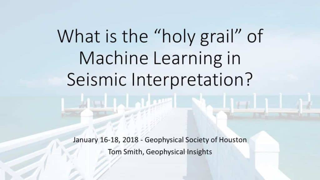 A few years ago, we had geophysics and geology – two distinct that were well defined. Then, geoscience came along, and it was an amalgam of geology and geophysics. Many people started calling themselves geoscientists as opposed “geologist” or “geophysicist”. But the changes weren’t quite finished. Along came a qualifying adjective, and that has to do with unconventional resource development or unconventional exploration. We understand how to do exploration, but unconventional has to do with understanding shale and finding sweet spots, but it is a type of exploration. By joining unconventional and resource development, we broaden what we do as professionals. However, the mindset of unconventional geophysics is really closer to mining geophysics than it is conventional exploration.