By Tao Zhao | Published with permission: SEG International Exposition and 88th Annual Meeting | October 2018
Introduction
With the rapid development in GPU computing and success obtained in computer vision domain, deep learning techniques, represented by convolutional neural networks (CNNs), start to entice seismic interpreters in the application of supervised seismic facies classification. A comprehensive review of deep learning techniques is provided in LeCun et al. (2015). Although still in its infancy, CNN-based seismic classification is successfully applied on both prestack (Araya-Polo et al., 2017) and poststack (Waldeland and Solberg, 2017; Huang et al., 2017; Lewis and Vigh, 2017) data for fault and salt interpretation, identifying different wave characteristics (Serfaty et al., 2017), as well as estimating velocity models (Araya-Polo et al., 2018).
The main advantages of CNN over other supervised classification methods are its spatial awareness and automatic feature extraction. For image classification problems, other than using the intensity values at each pixel individually, CNN analyzes the patterns among pixels in an image, and automatically generates features (in seismic data, attributes) suitable for classification. Because seismic data are 3D tomographic images, we would expect CNN to be naturally adaptable to seismic data classification. However, there are some distinct characteristics in seismic classification that makes it more challenging than other image classification problems. Firstly, classical image classification aims at distinguishing different images, while seismic classification aims at distinguishing different geological objects within the same image. Therefore, from an image processing point of view, instead of classification, seismic classification is indeed a segmentation problem (partitioning an image into blocky pixel shapes with a coarser set of colors). Secondly, training data availability for seismic classification is much sparser comparing to classical
image classification problems, for which massive data are publicly available. Thirdly, in seismic data, all features are represented by different patterns of reflectors, and the boundaries between different features are rarely explicitly defined. In contrast, features in an image from computer artwork or photography are usually well-defined. Finally, because of the uncertainty in seismic data, and the nature of manual interpretation, the training data in seismic classification is always contaminated by noise.
To address the first challenge, until today, most, if not all, published studies on CNN-based seismic facies classification perform classification on small patches of data to infer the class label of the seismic sample at the patch center. In this fashion, seismic facies classification is done by traversing through patches centered at every sample in a seismic volume. An alternative approach, although less discussed, is to use CNN models designed for image segmentation tasks (Long et al., 2015; Badrinarayanan et al., 2017; Chen et al., 2018) to obtain sample-level labels in a 2D profile (e.g. an inline) simultaneously, then traversing through all 2D profiles in a volume.
In this study, I use an encoder-decoder CNN model as an implementation of the aforementioned second approach. I apply both the encoder-decoder model and patch-based model to seismic facies classification using data from the North Sea, with the objective of demonstrating the strengths and weaknesses of the two CNN models. I conclude that the encoder-decoder model provides much better classification quality, whereas the patch-based model is more flexible on training data, possibly making it easier to use in production.
The Two Convolutional Neural Networks (CNN) Models
Patch-based model
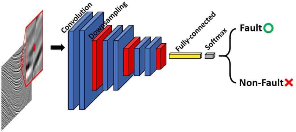
A basic patch-based model consists of several convolutional layers, pooling (downsampling) layers, and fully-connected layers. For an input image (for seismic data, amplitudes in a small 3D window), a CNN model first automatically extracts several high-level abstractions of the image (similar to seismic attributes) using the convolutional and pooling layers, then classifies the extracted attributes using the fully- connected layers, which are similar to traditional multilayer perceptron networks. The output from the network is a single value representing the facies label of the seismic sample at the center of the input patch. An example of patch-based model architecture is provided in Figure 1a. In this example, the network is employed to classify salt versus non-salt from seismic amplitude in the SEAM synthetic data (Fehler and Larner, 2008). One input instance is a small patch of data bounded by the red box, and the corresponding output is a class label for this whole patch, which is then assigned to the sample at the patch center. The sample marked as the red dot is classified as non-salt.
Encoder-decoder model
Encoder-decoder is a popular network structure for tackling image segmentation tasks. Encoder-decoder models share a similar idea, which is first extracting high level abstractions of input images using convolutional layers, then recovering sample-level class labels by “deconvolution” operations. Chen et al. (2018) introduce a current state-of-the-art encoder-decoder model while concisely reviewed some popular predecessors. An example of encoder-decoder model architecture is provided in Figure 1b. Similar to the patch-based example, this encoder-decoder network is employed to classify salt versus non-salt from seismic amplitude in the SEAM synthetic data. Unlike the patch- based network, in the encoder-decoder network, one input instance is a whole line of seismic amplitude, and the corresponding output is a whole line of class labels, which has the same dimension as the input data. In this case, all samples in the middle of the line are classified as salt (marked in red), and other samples are classified as non-salt (marked in white), with minimum error.
Application of the Two CNN Models
For demonstration purpose, I use the F3 seismic survey acquired in the North Sea, offshore Netherlands, which is freely accessible by the geoscience research community. In this study, I am interested to automatically extract seismic facies that have specific seismic amplitude patterns. To remove the potential disagreement on the geological meaning of the facies to extract, I name the facies purely based on their reflection characteristics. Table 1 provides a list of extracted facies. There are eight seismic facies with distinct amplitude patterns, another facies (“everything else”) is used for samples not belonging to the eight target facies.
| Facies number | Facies name |
| 1 | Varies amplitude steeply dipping |
| 2 | Random |
| 3 | Low coherence |
| 4 | Low amplitude deformed |
| 5 | Low amplitude dipping |
| 6 | High amplitude deformed |
| 7 | Moderate amplitude continuous |
| 8 | Chaotic |
| 0 | Everything else |
To generate training data for the seismic facies listed above, different picking scenarios are employed to compensate for the different input data format required in the two CNN models (small 3D patches versus whole 2D lines). For the patch-based model, 3D patches of seismic amplitude data are extracted around seed points within some user-defined polygons. There are approximately 400,000 3D patches of size 65×65×65 generated for the patch-based model, which is a reasonable amount for seismic data of this size. Figure 2a shows an example line on which seed point locations are defined in the co-rendered polygons.
The encoder-decoder model requires much more effort for generating labeled data. I manually interpret the target facies on 40 inlines across the seismic survey and use these for building the network. Although the total number of seismic samples in 40 lines are enormous, the encoder-decoder model only considers them as 40 input instances, which in fact are of very small size for a CNN network. Figure 2b shows an interpreted line which is used in training the network
In both tests, I randomly use 90% of the generated training data to train the network and use the remaining 10% for testing. On an Nvidia Quadro M5000 GPU with 8GB memory, the patch-based model takes about 30 minutes to converge, whereas the encoder-decoder model needs about 500 minutes. Besides the faster training, the patch-based model also has a higher test accuracy at almost 100% (99.9988%, to be exact) versus 94.1% from the encoder- decoder model. However, this accuracy measurement is sometimes a bit misleading. For a patch-based model, when picking the training and testing data, interpreters usually pick the most representative samples of each facies for which they have the most confidence, resulting in high quality training (and testing) data that are less noisy, and most of the ambiguous samples which are challenging for the classifier are excluded from testing. In contrast, to use an encoder-decoder model, interpreters have to interpret all the target facies in a training line. For example, if the target is faults, one needs to pick all faults in a training line, otherwise unlabeled faults will be considered as “non-fault” and confuse the classifier. Therefore, interpreters have to make some not-so-confident interpretation when generating training and testing data. Figure 2c and 2d show seismic facies predicted from the two CNN models on the same line shown in Figure 2a and 2b. We observe better defined facies from the encoder-decoder model compared to the patch- based model.
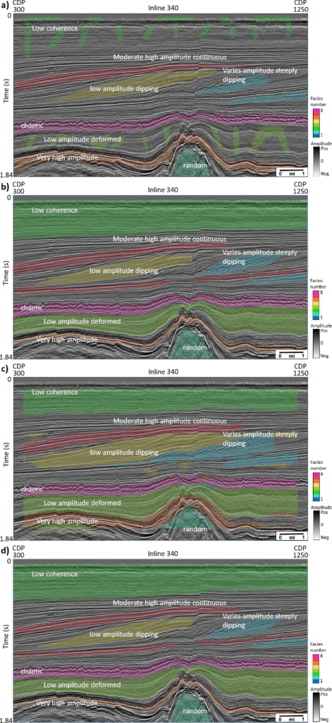
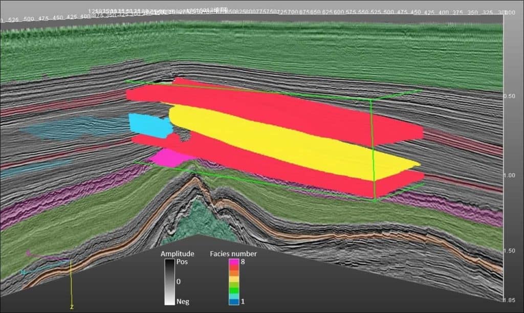
Figure 3 shows prediction results from the two networks on a line away from the training lines, and Figure 4 shows prediction results from the two networks on a crossline. Similar to the prediction results on the training line, comparing to the patch-based model, the encoder-decoder model provides facies as cleaner geobodies that require much less post-editing for regional stratigraphic classification (Figure 5). This can be attributed to an encoder-decoder model that is able to capture the large scale spatial arrangement of facies, whereas the patch-based model only senses patterns in small 3D windows. To form such windows, the patch-based model also needs to pad or simply skip samples close to the edge of a 3D seismic volume. Moreover, although the training is much faster in a patch-based model, the prediction stage is very computationally intensive, because it processes data size N×N×N times of the original seismic volume (N is the patch size along each dimension). In this study, the patch-based method takes about 400 seconds to predict a line, comparing to less than 1 second required in the encoder-decoder model.


Conclusion
In this study, I compared two types of CNN models in the application of seismic facies classification. The more commonly used patch-based model requires much less effort in generating labeled data, but the classification result is suboptimal comparing to the encoder-decoder model, and the prediction stage can be very time consuming. The encoder-decoder model generates superior classification result at near real-time speed, at the expense of more tedious labeled data picking and longer training time.
Acknowledgements
The author thanks Geophysical Insights for the permission to publish this work. Thank dGB Earth Sciences for providing the F3 North Sea seismic data to the public, and ConocoPhillips for sharing the MalenoV project for public use, which was referenced when generating the training data. The CNN models discussed in this study are implemented in TensorFlow, an open source library from Google.
References
Araya-Polo, M., T. Dahlke, C. Frogner, C. Zhang, T. Poggio, and D. Hohl, 2017, Automated fault detection without seismic processing: The Leading Edge, 36, 208–214.
Araya-Polo, M., J. Jennings, A. Adler, and T. Dahlke, 2018, Deep-learning tomography: The Leading Edge, 37, 58–66.
Badrinarayanan, V., A. Kendall, and R. Cipolla, 2017, SegNet: A deep convolutional encoder-decoder architecture for image segmentation: IEEE Transactions on Pattern Analysis and Machine Intelligence, 39, 2481–2495.
Chen, L. C., G. Papandreou, I. Kokkinos, K. Murphy, and A. L. Yuille, 2018, DeepLab: Semantic image segmentation with deep convolutional nets, atrous convolution, and fully connected CRFs: IEEE Transactions on Pattern Analysis and Machine Intelligence, 40, 834–848.
Chen, L. C., Y. Zhu, G. Papandreou, F. Schroff, and H. Adam, 2018, Encoder-decoder with atrous separable convolution for semantic image segmentation: arXiv preprint, arXiv:1802.02611v2.
Fehler, M., and K. Larner, 2008, SEG advanced modeling (SEAM): Phase I first year update: The Leading Edge, 27, 1006–1007.
Huang, L., X. Dong, and T. E. Clee, 2017, A scalable deep learning platform for identifying geologic features from seismic attributes: The Leading Edge, 36, 249–256.
LeCun, Y., Y. Bengio, and G. Hinton, 2015, Deep learning: Nature, 521, 436–444.
Lewis, W., and D. Vigh, 2017, Deep learning prior models from seismic images for full-waveform inversion: 87th Annual International Meeting, SEG, Expanded Abstracts, 1512–1517.
Long, J., E. Shelhamer, and T. Darrell, 2015, Fully convolutional networks for semantic segmentation: Proceedings of the IEEE Conference on Computer Vision and Pattern Recognition, 3431–3440.
Serfaty, Y., L. Itan, D. Chase, and Z. Koren, 2017, Wavefield separation via principle component analysis and deep learning in the local angle domain: 87th Annual International Meeting, SEG, Expanded Abstracts, 991–995.
Waldeland, A. U., and A. H. S. S. Solberg, 2017, Salt classification using deep learning: 79th Annual International Conference and Exhibition, EAGE, Extended Abstracts, Tu-B4-12.


