By Carolan Laudon, Sarah Stanley, Patricia Santogrossi | Published with permission: Unconventional Resources Technology Conference (URTeC 2019) | July 2019
Table of contents
-
Abstract
-
Introduction and preliminary work
-
Geologic Setting of the Niobrara and Surrounding Formations
-
Why Utilize Machine Learning
-
Machine Learning Data Preparation
-
Classification by Principal Component Analysis (PCA)
-
Self-Organzing Maps
-
SOM Results for the Survey and their Interpretation
-
A Marl Results
-
Codell Results
-
Structural Attributes
-
Conclusion
Abstract
Seismic attributes can be both powerful and challenging to incorporate into interpretation and analysis. Recent developments with machine learning have added new capabilities to multi-attribute seismic analysis. In 2018, Geophysical Insights conducted a proof of concept on 100 square miles of multi-client 3D data jointly owned by Geophysical Pursuit, Inc. (GPI) and Fairfield Geotechnologies (FFG) in the Denver-Julesburg Basin (DJ). The purpose of the study was to evaluate the effectiveness of a machine learning workflow to improve resolution within the reservoir intervals of the Niobrara and Codell formations, the primary targets for development in this portion of the basin.
The seismic data are from Phase 5 of the GPI/Fairfield Niobrara program in northern Colorado. A preliminary workflow which included synthetics, horizon picking and correlation of 28 wells was completed. The seismic volume was re-sampled from 2 ms to 1 ms. Detailed well time-depth charts were created for the Top Niobrara, Niobrara A, B and C benches, Fort Hays and Codell intervals. The interpretations, along with the seismic volume, were loaded into the Paradise® machine learning application, and two suites of attributes were generated, instantaneous and geometric. The first step in the machine learning workflow is Principal Component Analysis (PCA). PCA is a method of identifying attributes that have the greatest contribution to the data and that quantifies the relative contribution of each. PCA aids in the selection of which attributes are appropriate to use in a Self-Organizing Map (SOM). In this case, 15 instantaneous attribute volumes, plus the parent amplitude volume, were used in the PCA and eight were selected to use in SOMs. The SOM is a neural network-based machine learning process that is applied to multiple attribute volumes simultaneously. The SOM produces a non-linear classification of the data in a designated time or depth window.
For this study, a 60-ms interval that encompasses the Niobrara and Codell formations was evaluated using several SOM topologies. One of the main drilling targets, the B chalk, is approximately 30 feet thick; making horizontal well planning and execution a challenge for operators. An 8 X 8 SOM applied to 1 ms seismic data improves the stratigraphic resolution of the B bench. The neuron classification also images small but significant structural variations within the chalk bench. These variations correlate visually with the geometric curvature attributes. This improved resolution allows for precise well planning for horizontals within the bench. The 25 foot thick C bench and the 17 to 25 foot thick Codell are also seismically resolved via SOM analysis. Petrophysical analyses from wireline logs run in seven wells within the survey by Digital Formation; together with additional results from SOMs show the capability to differentiate a high TOC upper unit within the A marl which presents an additional exploration target. Utilizing 2D color maps and geobodies extracted from the SOMs combined with petrophysical results allows calculation of reserves for the individual reservoir units as well as the recently identified high TOC target within the A marl.
The results show that a multi-attribute machine learning workflow improves the seismic resolution within the Niobrara reservoirs of the DJ Basin and results can be utilized in both exploration and development.
Introduction and preliminary work
The Denver-Julesburg Basin is an asymmetrical foreland basin that covers approximately 70,000 square miles over parts of Colorado, Wyoming, Kansas and Nebraska. The basin has over 47,000 oil and gas wells with a production history that dates back to 1881 (Higley, 2015). In 2009, operators in the Wattenberg field began to drill and complete horizontal wells in the chalk benches of the Niobrara formation and within the Codell sandstone. As of October 2018, approximately 9500 horizontal wells have been drilled and completed within Colorado and Wyoming in the Niobrara and Codell formations (shaleprofile.com/2019/01/29/niobrara-co-wy-update-through-october-2018).
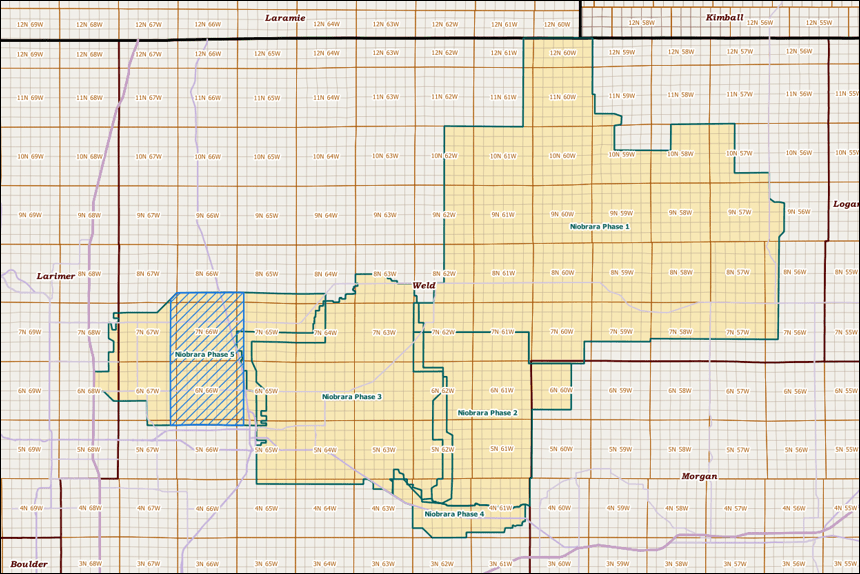
The transition to horizontal drilling necessitated the acquisition of modern, 3D seismic data (long offset, wide azimuth) to properly image the complex faulting and fracturing within the basin. In 2011, Geophysical Pursuit, Inc., in partnership with the former Geokinetics Inc., embarked on a multi-year, multi-client seismic program that ultimately resulted in the acquisition of 1580 square miles of contiguous 3D seismic data. In 2018, Geophysical Pursuit, Inc. (GPI) and joint-venture partner Fairfield Geotechnologies (FFG) provided Geophysical Insights with seismic data in the Denver-Julesburg Basin to conduct a proof of concept evaluation of the effectiveness of a machine learning workflow to improve resolution within the reservoir intervals of the Niobrara and Codell formations, currently the primary targets for development in this portion of the basin. The GPI/FFG seismic data analyzed are 100 square miles from the Niobrara Phase 5 multi-client 3D program in northern Colorado (Figure 1). Prior to the machine learning workflow, a preliminary interpretation workflow was carried out, that included synthetics, horizon picking and well correlation on 28 public wells with digital data. The seismic volume was resampled from 2 ms to 1 ms. Time depth charts were made with detailed well ties for the Top Niobrara, Niobrara A, B, and C benches, Fort Hays and Codell. The interpretations, along with the re-sampled seismic amplitude volume, were loaded into the Paradise® machine learning application. The machine learning software has several options for computing seismic attributes, and two suites were selected for the study: standard instantaneous attributes and geometric attributes from the AASPI (Attribute Assisted Seismic Processing and Interpretation) consortium (http://mcee.ou.edu/aaspi/).
Geologic Setting of the Niobrara and Surrounding Formations
The Niobrara formation is late Cretaceous in age and was deposited in the Western Interior Seaway (Kaufmann, 1977). The Niobrara is subdivided into the basal Fort Hays limestone and the Smoky Hill member. The Smoky Hill member is further subdivided into three subunits informally termed Niobrara A, B, and C. These units consist of fractured chalk benches which are primary reservoirs with marls and shales between the benches which comprise source rocks and secondary reservoir targets. (Figure 2). The Niobrara unconformably overlies the Codell sandstone and is overlain by the Sharon Springs member of the Pierre shale.
The Codell is also late Cretaceous in age, and unconformably underlies the Fort Hays member of the Niobrara formation. In general, the Codell thins from north to south due to erosional truncation (Sterling, Bottjer and Smith, 2016). In the study area, the thickness of the Codell ranges from 18 to 25 feet. Lewis (2013) inferred an eastern provenance for the Codell with a limited area of deposition or subsequent erosion through much of the DJ Basin. Based upon geochemical analyses, Sterling and others (2016) state that hydrocarbons produced from the Codell are sourced from the Niobrara, primarily the C marl, and the thermal maturity provides evidence of migration into the Codell. The same study found that oil produced from the Niobrara C chalk was generated in-situ.
Figure 2 (Sonnenberg, 2015) shows a generalized stratigraphic column and a structure map for the Niobrara in the DJ Basin along with an outline of the DJ basin and the location of the Wattenberg Field within which the study area is contained.
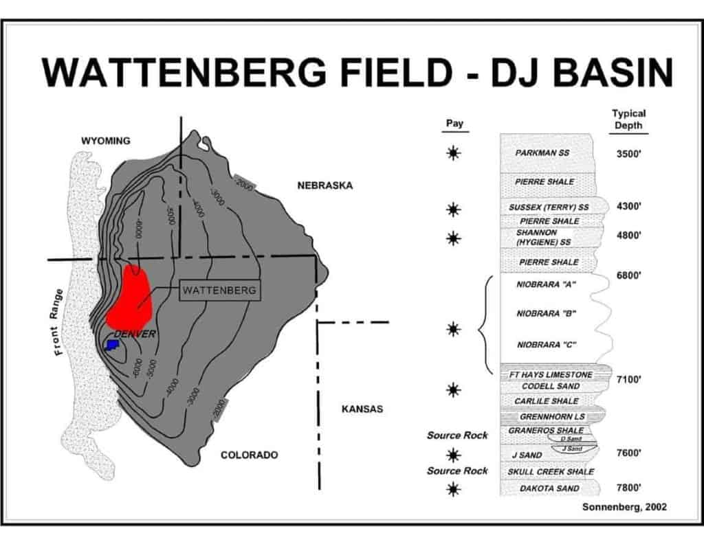
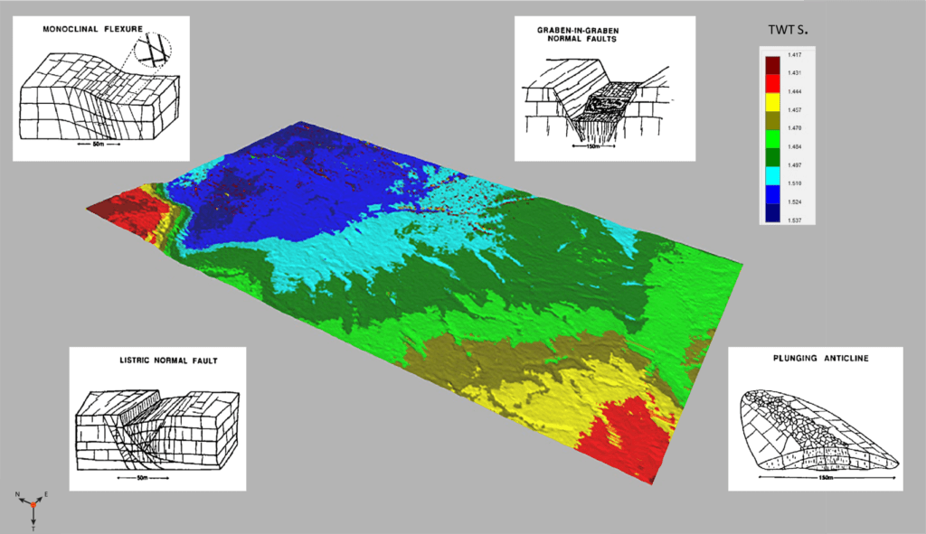
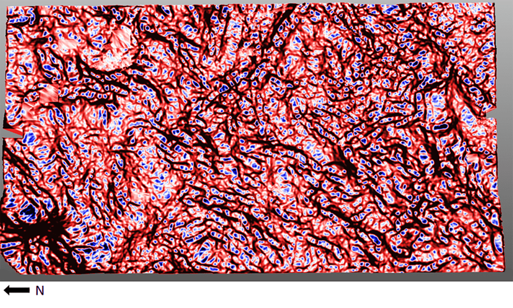
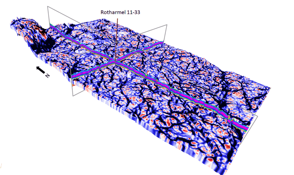
Figure 3 shows the structural setting of the Niobrara in the study area, as well as types of fractures which can be expected to provide storage capacity and permeability for reservoirs within the chalk benches (Friedman and others, 1992). The study area covers approximately 100 square miles and shows large antiforms on the western edge. The area is normally faulted with most faults trending northeast to southwest. The Top Niobrara time structure also shows extensive small-scale structural relief which is visualized in a curvature attribute volume as shown in Figure 4. This implies that a significant amount of fracturing is present within the Niobrara.
Meissner and others (1984) and Landon and others (2001) have stated that the Niobrara formation kerogen is Type-II and oil-prone. Landon and others, and Finn and Johnson (2005) have also stated that the DJ basin contains the richest Niobrara source rocks with TOC contents reaching eight weight percent. Niobrara petroleum production is dependent on fractures in the hard, brittle, carbonate-rich zones. These zones are overlain and/or interbedded with soft, ductile marine shales that inhibit migration and seal the hydrocarbons in the fractured zones.
Why Utilize Machine Learning?
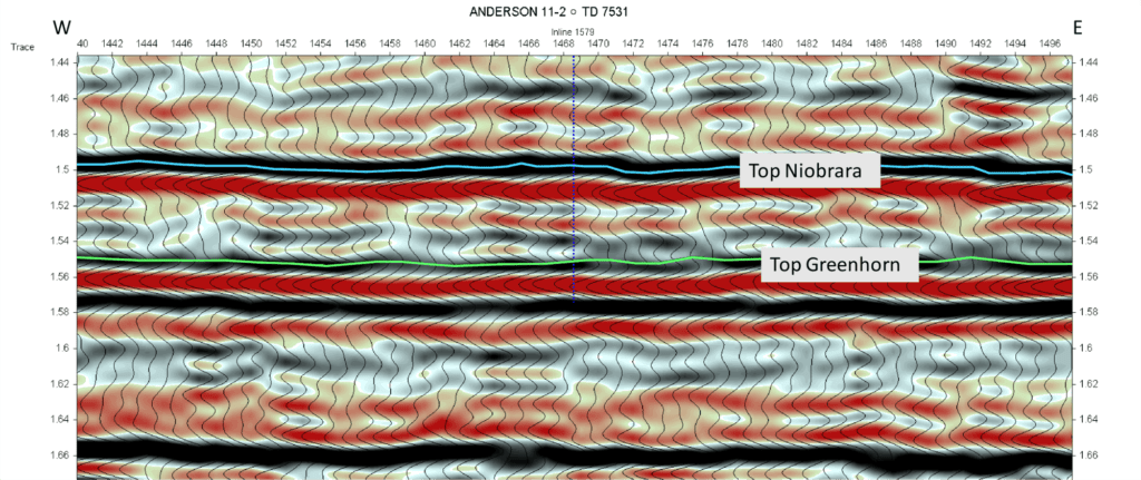
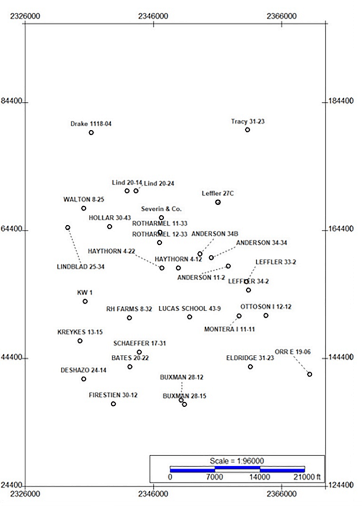
In the study area, the Niobrara to Greenhorn section is represented in approximately 60 milliseconds of two-way travel time in the seismic data. Figure 5 shows an amplitude section through a well within the study area. Figure 6 is an index map of wells used in the study with the Anderson 11-2 well highlighted in red. It is apparent that the top Niobrara is a well resolved positive amplitude or peak which can be picked on either a normal amplitude section or an instantaneous phase display. The individual units within the Niobrara A bench, A marl, B bench, B marl, C bench, C marl, Fort Hays and Codell present a significant challenge for an interpreter to resolve using only one or two attributes. The use of simultaneous multiple seismic attributes holds promise to resolve thin beds and a machine learning approach is one methodology which has been documented to successfully resolve stratigraphy below tuning (Roden and others, 2015, Santogrossi, 2017).
Machine Learning Data Preparation
The Niobrara Phase 5 3D data used for this study consisted of a 32-bit seismic amplitude volume that covers approximately 100 square miles. The survey contained 5.118 seconds of data with a bin spacing of 110 feet. Machine learning classifications benefit from sharper natural clusters of information through one level of finer trace sampling. Machine learned seismic resolution also benefits from sample-by-sample classification when compared to conventional wavelet analysis. Therefore, the data were upsampled to 1 ms from its original 2 ms interval by Geophysical Insights. The 1 ms amplitude data were used for seismic attribute generation.
Focus should be placed on the time interval that encompasses the geologic units of interest. The time interval selected for this study was 0.5 seconds to 2.2 seconds.
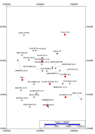
A total of 44 digital wells were obtained, 40 of which were within the seismic survey.
Classification by Principal Component Analysis (PCA)
Multi-dimensional analysis and multi-attribute analysis go hand in hand. Because individuals are grounded in three-dimensional space, it is difficult to visualize what data in a higher number dimensional space looks like. Fortunately, mathematics doesn’t have this limitation and the results can be easily understood with conventional 2D and 3D viewers.
Working with multiple instantaneous or geometric seismic attributes generates tremendous volumes of data. These volumes contain huge numbers of data points which may be highly continuous, greatly redundant, and/or noisy. (Coleou et al., 2003). Principal Component Analysis (PCA) is a linear technique for data reduction which maintains the variation associated with the larger data sets (Guo and others, 2009; Haykin, 2009; Roden and others, 2015). PCA has the ability to separate attribute types by frequency, distribution, and even character. PCA technology is used to determine which attributes to use and which may be ignored due to their very low impact on neural network solutions.
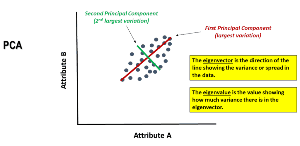
Figure 7 illustrates the analysis of a data cluster in two directions offset by 90 degrees. The first principal component (eigenvector 1) analyses the data cluster along the longest axis. The second principal component (eigenvector 2) analyses the data cluster variations perpendicular to the first principal component. As stated in the diagram, each eigenvector is associated with an eigenvalue which shows how much variance is in the data.
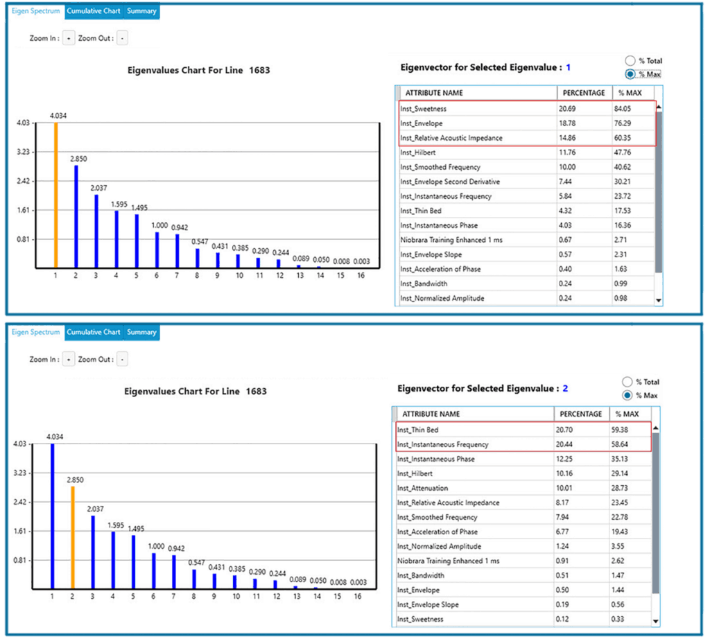
Eigenvectors and eigenvalues from inline 1683 were consistently used for Principal Component Analysis because line 1683 bisected the deepest well in the study area. The entire pre-Niobrara, Niobrara, Codell, and post-Niobrara depositional events were present in the borehole.
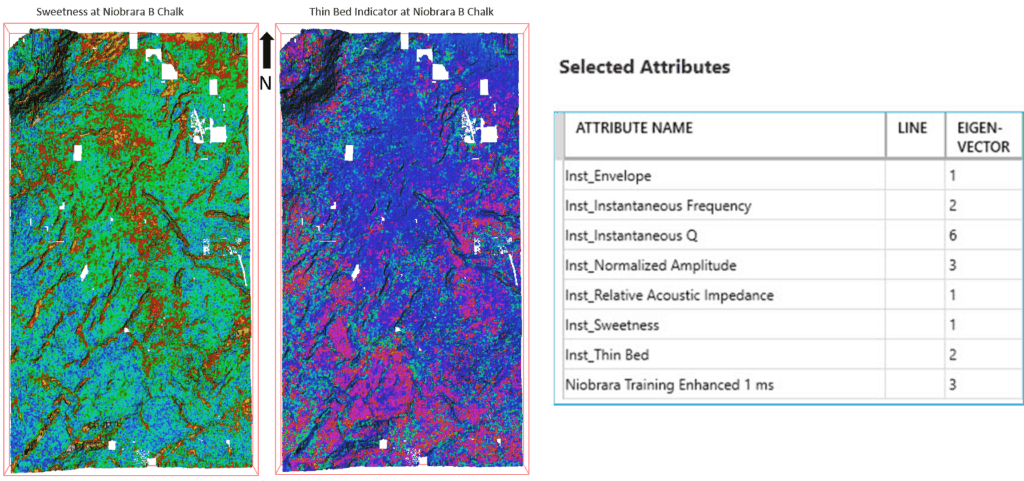
PCA results for the first two eigenvectors for the interval Top Niobrara to Top Greenhorn are shown in Figure 8. Results show the most significant attributes in the first eigenvector are Sweetness, Envelope, and Relative Acoustic Impedance; each contributes approximately 60% of the maximum value for the eigenvector. PCA results for the second eigenvector show Thin Bed and Instantaneous Frequency are the most significant attributes. Figure 9 shows instantaneous attributes from the first eigenvector (sweetness) and second eigenvector (thin bed indicator) extracted near the B chalk of the Niobrara. The table shown in Figure 9 lists the instantaneous attributes that PCA indicated contain the most significance in the survey and the eigenvector associated with the attribute. This selection of attributes comprises a ‘recipe’ for input to the Self-Organizing Maps for the interval Niobrara to Greenhorn.
Self-Organzing Maps
Teuvo Kohonen, a Finnish mathematician, invented the concepts of Self-organizing Maps (SOM) in 1982 (Kohonen, T., 2001). Self-Organizing Maps employ the use of unsupervised neural networks to reduce very high dimensions of data to a scale that can be easily visualized (Roden and others, 2015). Another important aspect of SOMs is that every seismic sample is used as input to classification as opposed to wavelet-based classification.
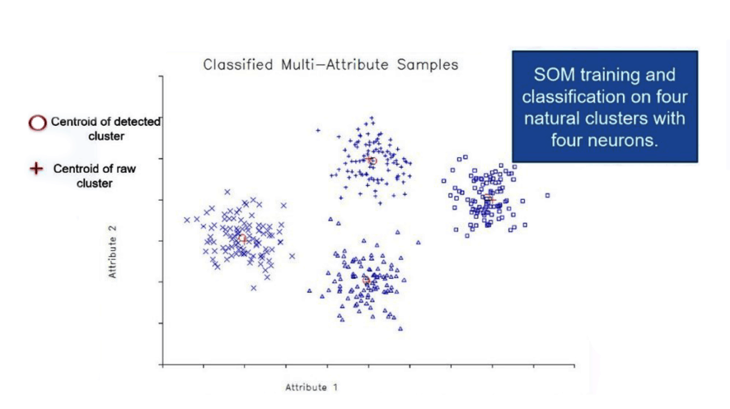
Figures 10 and 11 illustrate classification by SOM. Within the 3D seismic survey, samples are first organized into attribute points with similar properties called natural clusters in attribute space. Within each cluster new, empty, multi-attribute samples, named neurons, are introduced. The SOM neurons will seek out natural clusters of like characteristics in the seismic data and produce a 2D mesh that can be illustrated with a two- dimensional color map.
In other words, the neurons “learn” the characteristics of a data cluster through an iterative process (epochs) of cooperative then competitive training. When the learning is completed each unique cluster is assigned to a neuron number and each seismic sample is now classified (Smith, 2016).
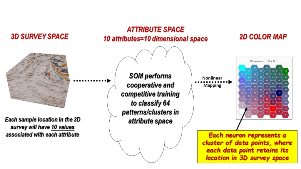
Note that the two-dimensional color map in Figure 11 shows an 8X8 topology. Topology is important. The finer the topology of the two-dimensional color map the finer the data clusters associated with each neuron become. For example: an 8X8 topology distributes 64 neurons throughout an attribute set, while a 12X12 topology distributes 144 neurons. Finer topologies help to refine variations in lithologies, porosity, and other reservoir characteristics. Although there is no theoretical limit to a two-dimensional map topology, experience has shown that there is a practical limit to the number of neuron topologies for geological resolution. Conversely, a coarser neuron topology is associated with much larger data clusters and helps to define structural features. For the Niobrara project an 8X8 topology appeared to give the best stratigraphic resolution for instantaneous attributes and a 5X5 topology resolved the geometric attributes most effectively.
SOM Results for the Survey and their Interpretation
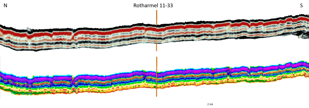
The SOM topology selected to best resolve the sub-Niobrara stratigraphy from the eight instantaneous attributes is an 8X8 hexagonal which yields 64 individual neurons. The SOM interval selected was Top Niobrara to Top Greenhorn. The next sequence of figures highlights the improved resolution provided by the SOM when compared to the original amplitude data. Figure 12 shows a north-south inline through the survey and through the Rotharmel 11-33 well which was one of the wells selected for petrophysical analysis. The original amplitude data is shown along with the SOM result for the interval.
The next image, Figure 13, zooms into the SOM and highlights the correlation with lithology from petrophysical analysis. The B chalk is noted by a stacked pattern of yellow-red-yellow neurons, with the red representing the maximum carbonate content within the middle of the chalk bench.
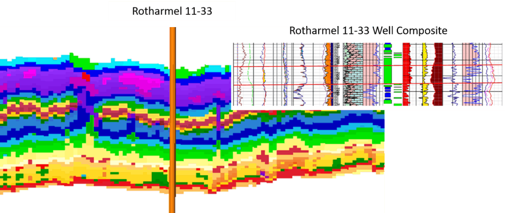
One can see on the SOM the sweet spot within the B chalk and that there is a fair amount of small-scale structural relief present. These results aid in the resolution of structural offset within the reservoir away from well control which is critical for staying in a 20 to 30 foot zone when drilling horizontally. Each classified sample is 1 ms in thickness which converted to depth equates to roughly 7 feet.
Figure 14 shows the K2 curvature attribute co-rendered with the SOM results in vertical sections. The Rotharmel 11-33 is at the intersection of the vertical sections. The curvature is extracted at the middle of the B chalk and shows good agreement with the SOM. The entire B bench is represented by only 5-6 ms of seismic data.
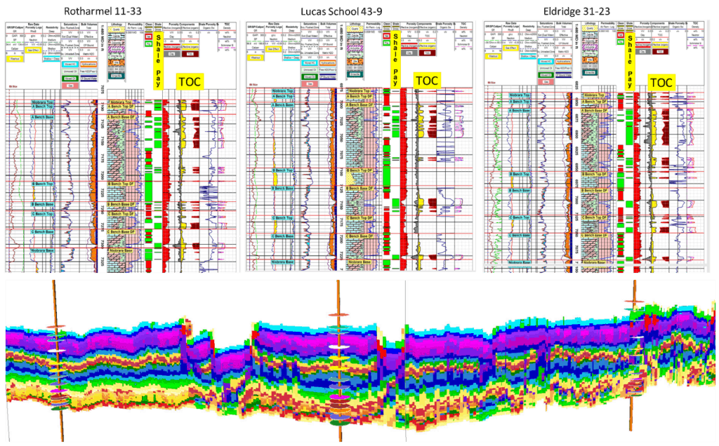
A Marl Results
Seven wells within the survey were sent to a third party for petrophysical analysis (Figure 15). The analysis identified zones of interest within the Niobrara marls which are typically considered source rocks. The calculations show a high TOC zone in the upper A marl which the analysis identifies as shale pay (Figure 16). A seismic cross-section of the 8X8 instantaneous SOM (Figure 16) through the three wells depicted shows that this zone is well imaged. The neurons can be isolated and volumetric calculations derived from the representative neurons.
Codell Results
The Codell sandstone in general and within the study area shows more heterogeneity in reservoir properties than the Niobrara chalk benches. The petrophysical analysis on 7 wells shows net pay ranging from zero feet to three feet. The gross thickness ranges from 17 feet to 25 feet. The SOM results reflect this heterogeneity, resolve the Codell gross interval throughout most of the study area, and thus, can be useful for horizontal well planning.
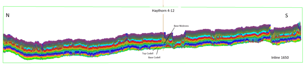
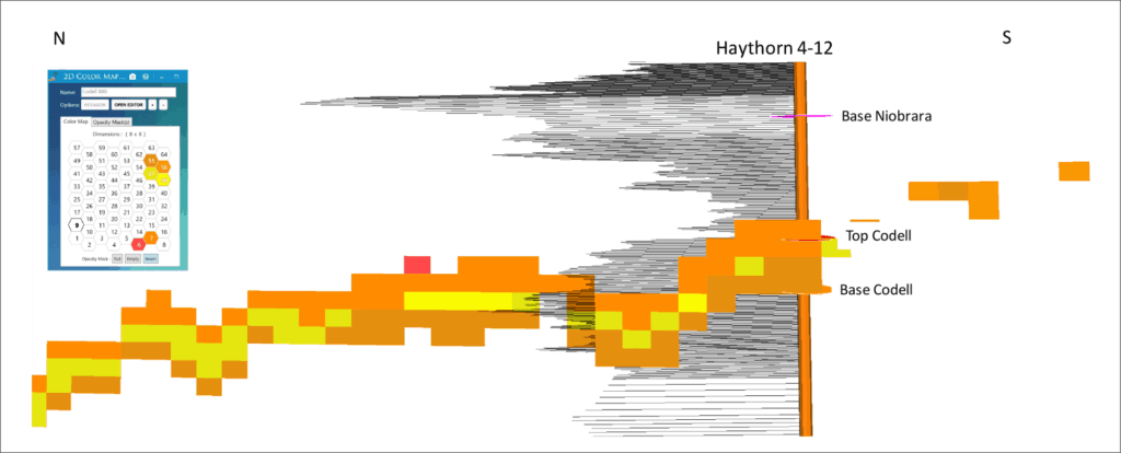
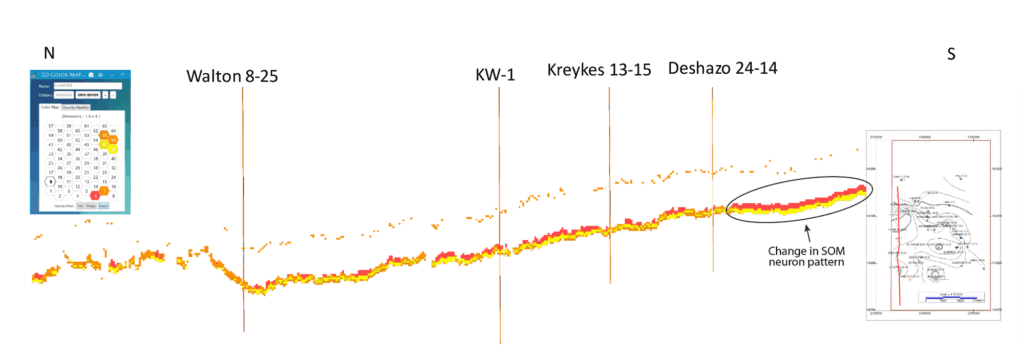
Figures 17 and 18 shows inline 60 through a well with the Top Niobrara to Greenhorn 8X8 SOM results. The 2D color map has been manipulated to emphasize the lower interval from approximately base Niobrara through the Codell. Figure 18 zooms into the well and shows the specific neurons associated with the Codell interval. Figures 19 shows a N-S traverse through four wells again with the Codell interval highlighted through use of a 2D color map. The western and southwest areas of the survey show a much more continuous character to the classification with only two neurons representing the Codell interval (6 and 48). Figure 20 shows both the N-S traverse and a crossline through the anomaly.
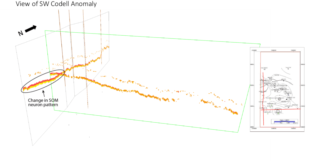
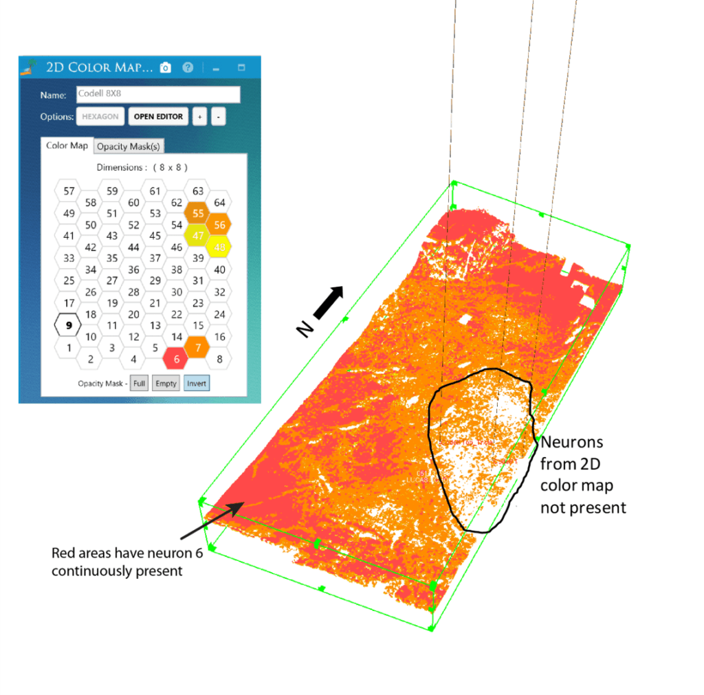
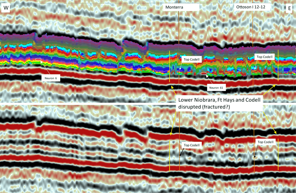
Unfortunately, vertical well control was not available through this southwestern anomaly. To examine the extent of individual neurons within the SOM at Codell level, the next image, Figure 21, shows a 3D view of the isolated Codell neurons. The southwest anomaly is apparent as well as similar anomalies in the northern portion of the survey. What is also immediately apparent is that in the east-central portion of the survey, the Codell is not represented by the six neurons (6,7,47, 48, 55, 56) previously used to isolate it within the volume. Figure 22 takes a closer look at the SOM results through this area and also utilizes the original amplitude data. Both the SOM and the amplitude data show a change in character throughout the entire section, but the SOM results only change significantly in the lower Niobrara to Greenhorn portion of the interval.
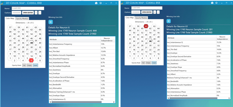
The machine learning application has a feature in which individual neurons can be queried for statistics on how individual seismic attributes contribute to the cluster which makes up the neuron. Queries were done on all of the neurons within the Codell and shown are the results for neuron 6 which is one of 2 neurons characteristic of the southwestern Codell anomaly and on neuron 61in the area where the SOM changes significantly in Figure 23. Neuron 6 has equal contributions from Instantaneous Frequency, Hilbert, Thin Bed, and Relative Acoustic Impedance. Neuron 61 shows Instantaneous Q as the top attribute which is consistent with the interpretation of the section being structurally disturbed or highly fractured.
Structural Attributes
The machine learning workflow can be applied to geometric attributes. PCA and SOM need to be run separately from the instantaneous attributes since PCA assumes a Gaussian distribution of the attributes. This assumption doesn’t hold for geometric attributes but the SOM process does not assume any distribution and thus still finds patterns in the data. To produce a structural SOM, four attributes were selected from PCA: Curvature_K1, Similarity, Energy Ratio, Texture Entropy, and Texture Homogeneity. These were combined with the original amplitude data to generate SOMs from the Top Niobrara to Top Greenhorn interval. Several SOM topologies were generated with geometric attributes and a 5X5 yielded good results. Figure 24 shows the geometrical SOM results at the Top Niobrara, B bench, and Codell. The Top Niobrara level shows major faults, but not nearly as much structural disturbance as the mid-Niobrara B bench or the Codell level. The eastern part of the survey where the instantaneous classification changed also shows significant differences between the B bench and Codell and agrees with the interpretation that this is a highly fractured area for the lower Niobrara and Codell. The B bench appears more structurally disrupted than the Top Niobrara but shows fewer areal changes compared to Codell. Pressure and production data could help confirm how these features relate to reservoir quality.
Conclusion
Seismic multi-attribute analysis has always held the promise of improving interpretations via the integration of attributes which respond to subsurface conditions such as stratigraphy, lithology, faulting, fracturing, fluids, pressure, etc. Machine learning augments traditional interpretation and attribute analysis by utilizing attribute space to simultaneously classify suites of attributes into sample based, high dimension clusters that are subsequently visualized and further interpreted in the 3D seismic survey. 2D colormaps aid in their interpretation and visualization.
In the DJ Basin, we have resolved the primary reservoir targets, the Niobrara chalk benches and the Codell formation, represented within approximately 60 ms of data in two-way time, to the level of one to five neurons which is approximately 7 to 35 feet in thickness. Structural SOM classifications with a suite of geometric attributes better image the complex faulting and fracturing and its variations throughout the reservoir interval. The classification volumes are designed to aid in drilling target identification, reserves calculations and horizontal well planning.
References
Coleou, T., M. Poupon, and A. Kostia, 2003, Unsupervised seismic facies classification: A review and comparison
of techniques and implementation: The Leading Edge, 22, 942–953, doi: 10.1190/1.1623635.
Finn, T. M. and Johnson, R. C., 2005, Niobrara Total Petroleum System in the Southwestern Wyoming Province, Chapter 6 of Petroleum Systems and Geologic Assessment of Oil and Gas in the Southwestern Wyoming Province, Wyoming, Colorado, and Utah, USGS Southwestern Wyoming Province Assessment Team, U.S. Geological Survey Digital Data Series DDS–69–D.
Guo, H., K. J. Marfurt, and J. Liu, 2009, Principal component spectral analysis: Geophysics, 74, no. 4, p. 35–43.
Haykin, S., 2009, Neural networks and learning machines, 3rd ed.: Pearson.
Kauffman, E.G., 1977, Geological and biological overview— Western Interior Cretaceous Basin, in Kauffman, E.G., ed., Cretaceous facies, faunas, and paleoenvironments across the Western Interior Basin: The Mountain Geologist, v. 14, nos. 3 and 4, p. 75–99.
Kohonen, T., 2001, Self-organizing maps: Third extended addition, Springer, Series in Information Services, Vol. 30.
Landon, S.M., Longman, M.W., and Luneau, B.A., 2001, Hydrocarbon source rock potential of the Upper Cretaceous Niobrara Formation, Western Interior Seaway of the Rocky Mountain region: The Mountain Geologist, v. 38, no. 1, p. 1–18.
Lewis, R.K., 2013, Stratigraphy and Depositional Environments of the Late Cretaceous (Late Turonian) Codell Sandstone and Juana Lopez Member of the Carlile Shale, Southeast Colorado: Colorado School of Mines MS Thesis, 190 p.
Longman, M.W., Luneau, B.A., and Landon, S.M., 1998, Nature and distribution of Niobrara lithologies in the Cretaceous Western Interior Seaway of the Rocky Mountain Region: The Mountain Geologist, v. 35, no. 4, p. 137–170.
Luneau, B., Longman, M., Kaufman, P., and Landon, S., 2011, Stratigraphy and Petrophysical Characteristics of the Niobrara Formation in the Denver Basin, Colorado and Wyoming, AAPG Search and Discovery Article #50469.
Meissner, F.F., Woodward, J., and Clayton, J.L., 1984, Stratigraphic relationships and distribution of source rocks in the greater Rocky Mountain region, in Woodward, J., Meissner, F.F., and Clayton, J.L., eds., Hydrocarbon source rocks of the greater Rocky Mountain region: Rocky Mountain Association of Geologists Guidebook, p. 1–34.
Molenaar, C.M., and Rice, D.D., 1988, Cretaceous rocks of the Western Interior Basin, in Sloss, L.L., ed., Sedimentary cover-North American craton, U.S.: Geological Society of America, The Geology of North America, v. D–2, p. 77–82.
Roden, R., Smith, T., and Sacrey, D., 2015, Geologic pattern recognition from seismic attributes: Principal component analysis and self-organizing maps, Interpretation, Vol. 3, No. 4, p. SAE59-SAE83.
Santogrossi, P., 2017, Classification/Corroboration of Facies Architecture in the Eagle Ford Group: A Case Study in Thin Bed Resolution, URTeC 2696775, doi 10.15530-urtec-2017-<2696775>.
Smith, T., 2016, Why SOM is an Appealing Learning Machine, Internal Geophysical Insights Paper.
Sonnenberg, S.A., 2015. Geologic Factors Controlling Production in the Codell Sandstone, Wattenberg Field, Colorado. URTeC Paper 2145312 presented at the Unconventional Resources Technology Conference, San Antonio, TX, July 20-22.
Sonnenberg, S.A., 2015. New reserves in an old field, the Niobrara/Codell resource plays in the Wattenberg Field, Denver Basin, Colorado. EAGE First Break, v. 33, p. 55-62.
Sterling, R., Bottjer, R. and Smith, K., 2016, Codell SS, A review of the Northern DJ oil resource play Laramie County, WY and Weld, County, CO, AAPG Search and Discovery Article #10754.