Summary
Convolutional Neural Networks (CNN)-based fault detection method is an emerging technology that shows great promise for the seismic interpreter. One of the more successful deep learning CNN methods uses synthetic data to train a CNN model. Although the synthetics are all normal faults, a common CNN practice is to augment the training data by rotating and flipping each image. Different types of noise are added to the synthetics to allow the algorithm to learn to see through the noise as a human interpreter does. A more traditional fault analysis workflows is based on seismic attributes and image processing. In contrast to CNN, the image processing “convolutions” have been predetermined based on concepts of signal analysis In this paper, we build a CNN architecture to predict faults from 3D seismic data, and then compare the results to those obtained using an image processing-based fault detection for datasets exhibiting different data quality.
Introduction
Traditional fault detection methods such as eigen-structure coherence (Gersztenkorn and Marfurt, 1999), gradient structure tensor (Bakker, 2002), energy-ratio similarity (Chopra and Marfurt, 2007), variance (Van Bemmel and Pepper, 200), and other variations of coherence algorithms have been widely used to highlight faults on 3D seismic data. However, because field seismic data also contain random noise and other stratigraphic features that exhibit similar discontinuous features, interpreters still need to spend time to differentiate faults from other incoherent anomalies. One way to address this is problem is to apply a filter to the coherence image. Randen et al. (2001) used a swarm intelligence algorithm, Cohen et al. (2006) a local fault extraction, Barnes (2006) eigenvector analysis of moment tensors followed by dilation and expansion, Wu and Hale (2015) an image processing technique, and Qi et al. (2018) an extension of Barnes workflow followed by an LoG filter and skeletonization.
CNN is a rapidly evolving technology that has applications that range from the recognition of faces for airport security to guiding decisions made by self-driving cars. CNN methods require large amounts of training data. For fault detection this implies a large collection of interpreted (or “labeled”) faults. Over the past three years Huang et al. (2017), Guo et al. (2018), Zhao and Mukhopadhyay (2018), Xiong et al. (2018), Li et al. (2019), Zhao (2019), and Wu et al. (2018, 2019) have shown that CNN can be trained to detect faults, differentiating them from other non-fault discontinuities in the seismic data.
In this paper, we build a deep learning U-net convolutional neural network architecture and apply it to predict faults from two datasets. The first dataset was acquired from offshore New Zealand and contains many vertical normal faults. The second data set is from onshore Gulf of Mexico and exhibits listric faults. We then analyze the same data set using a more traditional seismic attribute/fault enhancement/skeletonization workflow described by Qi et al. (2017 and 2018). We then compare the two results and draw preliminary conclusions.
The CNN-based fault detection workflow
There are several tasks required in CNN image classification and segmentation. First, we need to train the network, using a suite of small 3D volumes that are “labeled” as to whether or not the exhibit faulting. The direct way to construct such training data is to have an interpreter manually pick faults on a seismic amplitude volume. The subsequent learning (such as a stochastic or mini-batch gradient descent) algorithm then evaluates and updates the internal CNN model parameters. However, using real seismic data to generate training data requires enormous amounts of data to work well. Generating a large amount of data from real seismic amplitude data for a given survey is very time consuming. Organizationally, capturing and labeling manually picked faults from conventional workflows requires a significant IT investment.
An alternative method is to generate the training data by creating faulted synthetic seismic amplitude volumes. An advantage of using synthetic data is that we can easily define the total number of training samples and the patch size used for each label, which is the sample size fed into a CNN model. In this paper, we build totally 250 3D synthetic seismic data volumes with patch size of 128×128×128. In each seismic data volume, parameters of fault dip, azimuth, displacement are randomly chosen to generate various faults. The reflectors and stratigraphic variations are also randomly generated by adding vertical planar shifts and multiple 2D Gaussian lateral folds. The seismic spectrum, noise, and bandwidth is additionally considered to vary across different training samples. We randomly generate reflector space and set the peak frequency of Ricker wavelet between 30 Hz to 50 Hz. Representative training samples are shown in Figure 1. The first training sample exhibits very high signal-to-noise ratio with limited lateral folding whereas the second training sample is noisy and its reflectors are strongly folded. Note the steeply dipping faults in the second synthetic seismic model are difficult to visually identify.
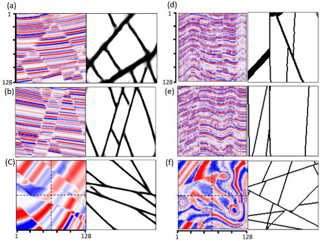
Because the training data is synthetic, we don’t need to perform additional data pre-conditioning. The only data augmentation we applied is data rotation to increase the number of models by rotating each training data by 90 degrees about the x, y, and z axes to create additional 3 volumes.
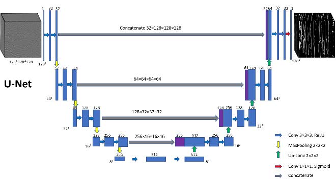
We build a modified U-Net architecture CNN model based on that proposed by Ronneberger et al. (2015). Following Ronneberger et al. (2015), Li et al. (2019), and Wu et al. (2019), we modify the number of filters and layers to evaluate the performance of a pre-trained model applications to various faults in different real datasets. Figure 2 show our U-Net architecture. We add nine blocks to extract features where each block contains two filter layers followed by a max pooling operator. The input is fed into a concatenation of different convolutional filters that are then fed into a decoder that localizes the feature. The final network consists of 18 convolutional 3×3×3 filter layers.
Unlike the typical autoencoder architecture that compresses data linearly, the U-Net architecture performs deconvolution, such that the output size of the U-Net architecture is equal to the input size. For this reason, we pad the output of each convolution to be the same size as the input. The maximum pooling sizes are 2×2×2. In the expansive part, the mathematically transposed convolutional operator is applied to perform upsampling of the feature maps using the learnable parameters. Our model only outputs one channel feature (there is or is not a fault) and uses a sigmoid activation function in the last layer. The loss function is binary cross entropy.
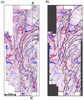
Image processing-based fault detection workflow
The image processing-based fault detection method we applied is the fault enhancement and skeletonization method described by Qi et al. (2017), Qi et al. (2018), and Lyu et al. (2019). This method inputs coherence and outputs fault probability that is iteratively filtered by energy-weighted directional Laplacian of a Gaussian (LoG) filters. The second-order moment tensor is built from the coherence attribute. The third eigenvector of the tensor represents the perpendicular direction of planar discontinuities. Discontinuities on coherence images are enhanced by the directional LoG filter through fault planes, and then skeletonized through the direction perpendicular to the fault planes.
Field data applications
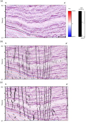
The first dataset is acquired from offshore New Zealand. We apply both CNN-based and image processing-based fault detection methods to compute fault probability. Figure 3 shows the comparison through vertical slices. Figure 3b shows seismic amplitude co-rendered with the image processing-based fault enhancement and skeletonization fault probability. Following Qi et al. (2018), we apply structure-oriented filtering, footprint suppression, and also compute multispectral coherence. The image processing- based fault probability exhibits good fault resolution. Note faults penetrating the middle chaotic mass transport deposits are also detected. Figure 3c shows the fault probability computed from the proposed CNN U-Net architecture. Note that the CNN fault probability image exhibits less incoherent noise but also other non-fault related discontinuities than the image processing-based fault probability image. Fault anomalies in both fault probability are sharp and continuous. The image processing-based fault probability is after skeletonization; thus, the faults in Figure 3b exhibit sharper than the faults in Figure 3c. Figure 4 shows a time slice comparison. Note faults in both fault probability volumes are very sharp and continuous.
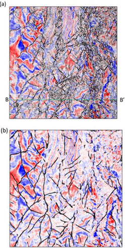
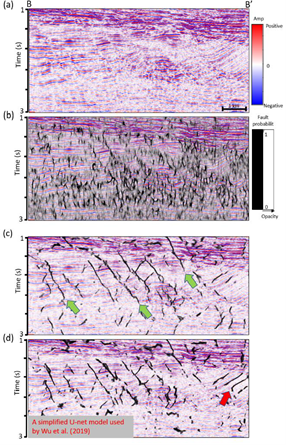
The major faults in our second test data are high angle dipping as well as soling out listric faults. This dataset is contaminated by migration artifacts and random noise resulting in a lower signal-to-noise ratio, especially in the deep area. Figure 5a show the vertical slices through the seismic amplitude volume. We first compute the image processing-based fault probability (Figure 5b). Because coherence maps all discontinuities including faults and stratigraphic discontinuities, those non-fault planar discontinuities are also enhanced through image processing workflow. The enhanced fault probability looks very noisy, although we are still able to recognize some major faults. Figure 3c show the CNN fault probability computed from the proposed U-Net architecture. The CNN fault probability exhibits cleaner fault anomalies but is also unable to map the soled-out part of the listric faults easily mapped by a human interpreter. Although CNN still shows non-fault planar discontinuities, more of these artifacts are rejected compared with the image processing fault probability. We also compare the proposed CNN architecture with a simplified CNN architecture. The major differences between the two CNN architecture are layer and filter number. Note that, the proposed CNN workflow shows slightly more continuous faults (indicated by green arrows in Figure 5) and less artifacts (indicated by red arrows). Figure 6 compares time slices through fault probability volumes computed using image processing and CNN.
Conclusions
In this paper, we have introduced a U-Net architecture to fault detection and compared it to a more traditional attribute/image processing fault mapping workflow. We trained the CNN model using synthetic seismic amplitude and fault labels computed for normal faults. The U-Net architecture CNN performs well on fault detection without any human-computer interactive work. The computational cost of training a CNN model is high, but extremely low on data prediction. In contrast the cost of the image processing- based method increases linearly with the size of the data volume. The CNN method was trained only to be sensitive to faults, resulting in two classes (fault and not-a-fault) which helped reject more stratigraphic discontinuities. The image processing fault probability exhibits a better performance in detecting vertical normal faults in a higher signal-to-noise dataset. The CNN method performs better than image processing method in detecting high angle dipping faults. Both methods failed to completely map listric faults. We anticipate that augmenting the training data with a suite of listric fault training models will improve the CNN performance.


