GSH-SEG Spring Symposium-Data Science and Geophysics: How Machine Learning and AI will Change Our Industry – Apr 27-28
The theme of Geophysical Society of Houston’s premier technical event was the application of the latest data science tools to solving geophysical problems.
The virtual symposium was held over two days and consisted of a keynote address, multiple speakers, and two exciting lunchtime events. The first was the traditional SEG Student Challenge Bowl competition. This was held online and featured the traditional battle between student geophysicists to be crowned the winner of the GSH Challenge Bowl and earn a place at the Challenge Bowl finals at the SEG annual symposium in the fall. The second event was the announcement of the winners of the Machine Learning Competition run by the Data Science & Machine Learning SIG and included an overview of the competition challenge, the announcement of the winner, and a presentation by the winning entry. The speaker lineup for the event included:
Key Note Speaker: Jake Umbriaco, Digital Platform and Services Manager, Subsurface – Chevron
Confirmed Speakers and Topics include:
- Aria Abubaker, Schlumberger – Machine Learning for Geoscience Applications
- Satinder Chopra, SamiGeo – Some Machine Learning Applications for Seismic Facies Classification
- Hugo Garcia, Geoteric – Automated Fault Detection from 3D Seismic using Artificial Intelligence
- Elive Menyoli, Emerson – Wavefield Separation via Principle Component Analysis and Deep learning in the Local Angle Domain
- Tom Smith, Geophysical Research, LLC (d/b/a Geophysical Insights) – The Scientific Universe from Square One to SOM
- Yuting Duan, Shell – Estimation of Time-lapse Timeshifts using Machine Learning
- Jon Downton, CGG – Predicting Reservoir Properties from Seismic and Well Data using Deep Neural Networks
- Wenyi Hu, AGT & UH – Progressive Transfer Learning for Low-Frequency Prediction in FWI
For more information, please click here.
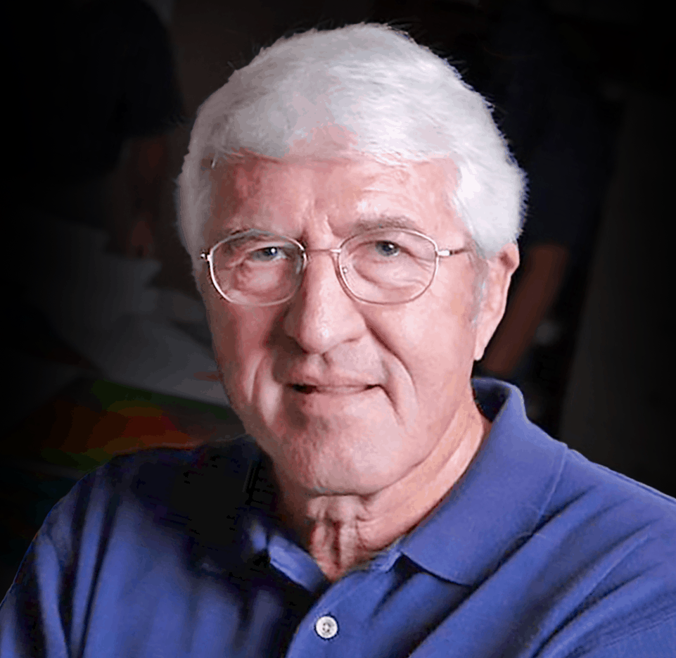
Dr. Thomas (“Tom”) A. Smith received a BS and MS degree in Geology from Iowa State University, and a Ph.D. in Geophysics from the University of Houston. His graduate research focused on a shallow refraction investigation of the Manson astrobleme. In 1971, he joined Chevron Geophysical as a processing geophysicist but resigned in 1980 to complete his doctoral studies in 3D modeling and migration at the Seismic Acoustics Lab at the University of Houston. Upon graduation with the Ph.D. in Geophysics in 1981, he started a geophysical consulting practice and taught seminars in seismic interpretation, seismic acquisition, and seismic processing. Dr. Smith founded Seismic Micro-Technology (SMT) in 1984 to develop PC software to support training workshops he was holding, which subsequently led to the development of the KINGDOM Software Suite for integrated geoscience interpretation.
In 2008, Dr. Smith founded Geophysical Insights, where he leads a team of geophysicists, geologists, and computer scientists in developing advanced technologies for fundamental geophysical problems. The company launched the Paradise® AI workbench in 2013, which uses Machine Learning, Deep Learning, and pattern recognition technologies to extract greater information from seismic and well data.
The Society of Exploration Geologists (SEG) recognized Dr. Smith’s work with the SEG Enterprise Award in 2000, and in 2010, the Geophysical Society of Houston (GSH) awarded him an Honorary Membership. Iowa State University (ISU) has recognized Dr. Smith throughout his career with the Distinguished Alumnus Lecturer Award in 1996, the Citation of Merit for National and International Recognition in 2002, and the highest alumni honor in 2015, the Distinguished Alumni Award. The University of Houston College of Natural Sciences and Mathematics recognized Dr. Smith with the 2017 Distinguished Alumni Award. In 2016, he was recognized by the Houston Geological Society (HGS) as a geophysicist who has made significant contributions to the field of geology.
Dr. Smith has been a member of the SEG since 1967 and is a professional member of SEG, GSH, HGS, EAGE, SIPES, AAPG, Sigma XI, SSA, and AGU. Dr. Smith served as Chairman of the SEG Foundation from 2010 to 2013. He currently serves on the SEG President-Elect’s Strategy and Planning Committee and the ISU Foundation Campaign Committee for Forever True, For Iowa State. The University of Houston College of Natural Sciences and Mathematics recognized Dr. Smith with the 2017 Distinguished Alumni Award.
Please contact us to receive more information on the Paradise AI workbench.
[forminator_form id=”34008″]

Dr. Tom Smith
Transcript
Dr. Tom Smith:
Sorry about the technical difficulties, everyone, but in a nutshell, what we’re going to be doing in these next 35 minutes, we are going to start with basics. And I hope that doesn’t switch you off, but we are going to start off with the basics, and the basic, scientifically, is a black box, and we’re going to follow the tracks of where that black box takes us to what I’m going to be calling the queen of statistics. So I’ll just leave it at that for a few minutes and let you figure out, “What in the world is Tom talking about, queen of statistics? What is that?” After we get to that point, we’re going to demonstrate how the queen of statistics works with our seismic data and how it will benefit our seismic interpretations, and we’ll conclude the presentation with three recent interpretations.
Let’s start off simply. We have a single US $1 bill, and we’re going to weigh it on an accurate scale, as you can see on the right. And we ask some simple questions after we get the number. We have a weight, we have a certain number, and we’re going to ask some simple questions, such as, well, do all US dollar bills weigh the same? Is the weight of a $5 bill heavier, and does the weight change with time? These are basic questions. And so to be sure about this, we go back and we weigh the bill a second time, and guess what? I can guarantee you that we will get a different value. Now, the legitimate thing to do would be to estimate the number of significant digits recorded by these two measurements or more, and that’s what we would report. We have a number of significant digits.
But let’s get at the heart of the matter a little bit better. Why are these two measurements different? That’s the question. Well, if we don’t have an answer to that, we legitimately and honestly must create something new, and that’s black box as you can see on the right side, down at the bottom there, we put the process in a black box. Why do we do that? Because we don’t have an explanation for the different values, two or more. To be honest about this, take this little experiment and we have to put a cloak around it and say, “It’s a black box. We just don’t know what to do about this situation.” We asked a simple question on our statistical events. Are they real or not?
Well, situations where we can’t make exact measurements, excuse me a second here. Where we can’t make exact measurements. For example, we have a box now and we have a single event which we then reduce to one value. And we ask the universe, “Hello out there. Is this black box repeatable?” And we go to our next round and try it again. And if we do this again and again and again and again, we repeat the process, same black box, but now I have a series of events. They’re causal events. One happens right after the other. So put a little square bracket around this and indicate that this is a set of values now, but they’re an ordered set, because we recorded the first time, second time, the third time, continuing on like that. So we repeat the process. Now that’s not the whole story, because we’re not real sure if that’s a single process, or maybe there’s more than one process inside a little black box.
We also have the possibility of coincident events. We’ll have a series of values there, but that will be at one instant of time, where we have multiple sensors hooked up and we have coincident events, so we can measure several items of the same event. And we have another set of values now, but they’re at one incident of time, and when we record this again and again and again, we change the brackets to a spiral set of values over there to indicate that it’s a little bit different. And we ask simply, is a universe determined or is it indeterminate? Kind of a basic question. Well, as I’m sure you know, statistics helps us to understand and make sense of an indeterminate universe. That’s the way it works. And it’s not only a value of course in all the sciences, and in particular geo science, but it helps us establish some predictability, and based upon that predictability, we can make some reasonable predictions. It’s a simple statement that we can’t know everything.
Well, we’ll start off here with this black box, as you can see on the right, single event. And we’re going to ask a series of questions here. Simple one, here’s a black box. And is there one process in the box or is there more than one? In other words, can that process in the black box be divided? Yes or no? Is there more than one process? Two or more? Well, are they independent of each other? We have another question. What is their independence? If one depends upon the other, how do they affect the results? Well, we study that with joint distributions. And does anything ever change across time? Do the values change over time? Well, if they do, or if they don’t, that’s the topic of sarcastic aspects of the statistics and how do they change over time?
Well, that’s another field, and that’s their [inaudible] of the statistics, and what triggers an event to happen in the first place, well that’s just the simple discovery. And if the box contains several processes, can we separate these into separate black boxes? Well, that’s our employment. The conclusion is, frankly, indeterminacy, it’s really a big topic. We’ll spend a couple of minutes here, starting at the roots of probability, which you may or may not realize, probability is not indeterminacy. It’s something more than that. Let’s figure that out. Probability involves chance. Chance is also not indeterminacy. Chance is the possibility of an event happening amongst all possible events.
And we have a gentleman over here on the right, Girolamo Cardano, 1501 to 1576. He worked on this area of something new, not just indeterminacy, and can’t do anything more about it. We’re working on the concept of probability and laid out the probability of each of all possible events. Each possible event has its own probability. And probability itself is bounded. It’s bounded by the sum of all possible probabilities, and that sum of the probabilities adds up to one. That is the probability of certainty. It’s one. And all probabilities, as I’m sure you know, are all less than one. The little tricky part about this that’s sometimes forgotten as we sort of skip right over it, is of all possible events. We need to be a little bit careful about that.
The measurements are several events that sometimes we take those to infinity, which in this case, is a mathematical approximation, but probabilities are not exact. And Girolamo Cardano is the father of probability. Let’s take a look at the whole concept here of the statistics of classification. We’re going to look at it the following way. Let’s read this together. The universe may be indeterminate because we don’t know everything, but through the mathematics of counting, we can exactly subdivide a finite set of objects into an exact number of subdivisions.
Notice the word exactly. We can exactly subdivide, and there’s an adjective there, and the exact number of subdivisions. The adjectives and the adverbs have something to do with simple counting. There’s a glimmer of hope in this world of chaos and indeterminacy. There is a little determinacy here, and that is because counting is the easiest type of mathematics around the simplest. There’s no integration here. There’s nothing associated with that of all. The most basic type of statistics, the most exact type of statistics is classification, because we have a whole ability to define counting and put objects in sets. We count those the way we want to count them. So without hesitation, we conclude statistical classification as a branch of statistics, as truly the queen of statistics. Fortunately, we’re finding in our machine learning that this classification process, the statistical classification is indeed meeting great success. We’re actually very fortunate with that. Now, if classification is good, is that all there is? And we continue to ask the questions, well, what does a classification model really look like?
Let’s take a look at the next step after just classification. And now let’s look at a special type of classification. This is self-organizing classification. Over on the left in sort of a dark red, as you can see there, is the town of Pavia, Italy. It’s in northern Italy. And if you look at the shape of this little province right there, it’s in north Italy up in this corner right here that I’m pointing at. Now, Girolamo Cardano taught at the University of Pavia, which by the way, is one of the oldest universities in the world. And Pavia is in the province of Lombardi, rich agricultural lands. And would you say that the regions of Lombardi are self-organized or not? Let’s see if we can sort of slide in what self-organizing is all about. Well, take a look at this. The probability that poor old professor Cardano, many years ago, our father of probability, he taught at the University of Pavia, but do you suppose he ever encountered the concept of self-organization or ever thought about it? Highly unlikely. In other words, the probability of Cardano and self-organization, probability is pretty close to zero.
Well, let’s sneak up a little closer on this and ask, well, what does self-organization really mean? How do we define it? Well, guess what? Here’s a perfect example. The people of Lombardi have self-organized themselves. So we are sneaking up on it. Self-organization categorizes common properties. So we can see even within the province of Lombardi, there are certain areas probably too rough to plow through. And there are other regions that are highly agriculture, smaller like that, and probably go to agricultural soil conditions and also the size of towns and things like that. You getting the idea? Okay, let’s move on then.
Self-organized learning. Aristotle, sorry, 384 to 322 BC, had a school of rhetoric and it was not only a school, but also a way of thinking. Deduction was born with the introduction of experimental learning. Aristotle taught that the world could be actively investigated, and think about that. That really is a profound thought. It’s a huge thought. Socrates, in an earlier time, 470 to 399 BC, taught that during his time, there was a school that he had put together, and that school is the dialectic method, which says a problem was broken down into parts. Parts are studied individually and conclusions are drawn, so the problem is simply solved by the sum of parts.
Whereas the later process of thinking of the world is by deduction. We work on one part A, we conclude B, and from B, we study it, conclude C, carry on like that. Each of these steps is a step in deduction. Socrates’ earlier school was a process of induction where you study the individual parts and put them all together. Understanding both of these types of thinking is fundamental for understanding self-organizing patterns and how these patents are going to be analyzed. By who? By us. It’s part duction and part induction. It’s both.
So in this new seismic interpretation methodology, the interpreter uses machine learning to find patterns in the data that may have otherwise gone undetected. That’s the beauty and the power of our machine learning processes. Machine learning delivers statistical bottles. This is a fundamental point, often overlooked. Machine learning delivers a statistical model. We need to think about it statistically and analyze it and interpret it statistically. The interpreter is allowed, by this perspective, to focus more on the processes and less on creative interpretation. The goal of this new cooperation between the interpreter and the machine remains the same. Let’s make better predictions. That’s the bottom line. We have a new set of tools to help us with this.
Now, there was a professor, University of Finland, I believe, Teuvo Kohonen, who statistically modeled different categories of data, and those that he analyzed, the relationships between the different objects was not, no. He modeled his machine learning on a two dimensional model of connected neurons inspired by the visual cortex in the back of our heads. Left side is to the right eye. And the right side, if you recall, is to the left eye. So mapping from the eye through the optic nerve, to the visual cortex, two parts. Now he observed that the different regions of the neural network ended up after their training in different general characteristics. So one part of the neural network had one set of general characteristics, other regions of a neural network had different characteristics. He coined this self-organizing map. SOM is a type of unsupervised neural network with coincidence events, using attributes all recorded at the same time, they are coincidence events, and they could be put into a simple spreadsheet of rows and columns. Now we may not use a real spreadsheet, but certainly, it can be organized this way.
Bottom line, SOM is a statistical classification model, and there is an evolutionary process here. There is an evolution of machine learning, starting from the machine learning, self-adaptation to self-organization, and even self-awareness. And let’s look at these different parts, so you can see what I’m really talking about here. Self-adaptation in that aspect, we have machine algorithms that adapt to specific characteristics of the data, and they store this information in a layered neural network. Straightforward. Use it all the time. Self-organization, the neural network itself is organized into patterns that can be evaluated and recognized and interpreted. And then finally, the third level is self-awareness. Well, that’s self-organizing neural networks that adapt not only to the data, but also to the environment. And this is the evolutionary process of machine learning neural networks from one to the other.
Let’s take a look at SOM as a statistical modeler. We’ll start off with some coincidence sampling. And at one instant of time, we record a bunch of properties, a bunch of attributes, simple as that. So one event is one sample, but we’re recording a series of measurements, if you will. And we do that for a bunch of different events and we group all those together and we call that one big set of a number of events. But each event is a series of that, of the attributes. We can slap all of this into an Excel spreadsheet, as we’ve done right here. And then we can run a SOM classification on this process. As I say, it’s unsupervised machine learning, and it will organize the data into classes, and we take a look at those. So this very simple minded result here is, is that we add to more columns to our spreadsheet right here. And we get not only the classification from this machine learning process, but also the probability, which is the goodness of fit.
So for example, that first event, which would be, say, the first line, and we might color that as class one, which would give that a color. That’s a gray, and the second one might be a blue. And then the third one might be an orange or something like that. Very simple concepts, straightforward to implement, and very interesting results to interpret. Well, let’s focus on, the SOM as a statistical model. It results from machine learning that trains, looks for natural clusters of information and attribute space. The process depends heavily on three basic things. It depends upon our choice of attributes, our choice of our neural network. And of course, it always depends upon our choice of training samples. After training the SOM, a neural network is a map of what we call winning neurons. After training, the SOM model can be used, that neural network can be used to classify all samples of interest.
A single sample is classified to its nearest winning neuron, which is the closest distance and attribute space in the SOM. Classified samples also have this goodness of fit and they address how close the winning neuron is to the sample where it lies in attribute space. Now, we could have an attribute space with two attributes and that’s all on a piece of paper. If we have eight attributes, 10 attributes, it’s eight or 10 dimensional space, not a problem for computer work. A winning neuron lies near the center of a natural cluster in attribute space. Let’s take a look at what that really implies. It really implies the following. A winning neuron lies next to the center of a natural cluster. And so we have natural clustering. So this element in the SOM corresponds to these samples, and then the one over here, these samples, et cetera, et cetera, et cetera. Very straightforward, leads us to some very interesting things.
And each sample can be analyzed and find out what is its classification probability? Is it a good fit or a poor fit? You have here 100 seismic traces of our four basic seismic reflection wavelets, and we’ll start off here with a low noise level. So we’re going from, say, low acoustic impedance to high, and with a symmetric wavelet, we then have a symmetric peak event going from low acoustic impedance to high. Single reflection [inaudible] positive. We also have a little acoustic impedance thin bed response, which is a trough over peak events and isometric. We have a high acoustic impedance thin bed, which is a peak over trough. And then finally, the last of the four basic. And that would be from a high acoustic impedance back to low, and that would be a symmetric trough event. Down at the bottom, you can see the SOM results of using the 100 traces here as training samples, and classification is laid on top using this color map down here in the lower right-hand corner.
We repeat the same process with the medium level of noise, and a little bit higher level of noise. These are the results. You can see that over on the left, whereas everything comes up very nicely, because we’ve added no noise, here we’ve got medium, and then higher level of noise. Notice that even with the higher level of noise, over here at the top of our four basic reflection events, we see trackable, certainly, easily trackable events of these four basic reflection wavelets.
Let’s take a look at the results in attribute space. In other words, for every seismic trace, we’ll have the amplitude and we’ll also have its Hilbert transform. And we plot every sample then in attribute space, because there’s only two, the amplitude in the Hilbert transform though, of course, we’ll plot as single points. And we have then a sample here, which would be a plus. And after SOM, we have a winning neuron. And that’s with 100 seismic samples for low levels of noise, medium levels of noise, and higher levels of noise.
And you can see here, but in all cases, even for the higher level of noise, we have a cluster of samples in attribute space, which cluster around the seismic sample. Now let’s take a look at this a little closer. Here’s a synthetic seismogram, and I’m talking about a seismogram trace. It’s really got two parts. It’s got the real trace and the transform. Here’s the reflection coefficients, single reflection coefficient, the two couplets, and then back to the single again. And we plot these results after the SOM classification, 100 synthetic seismograms with medium noise, and you can see the results here. And then if we go back to the seismic traces themselves and categorize those, fast them, now these are the results.
So if we go to this first one, symmetric peak event, we know that the value of the real trace is a maximum. So it’s a large amplitude value, and we know that it’s a zero crossing of the Hilbert transform, which is a nine degrees ratio from the real trace. So the Hilbert transform is zero. And that means is that the Hilbert transform is zero, large positive amplitude. In other words, that sample would plot over here somewhere. We also have, then, the winning neuron classified samples as these two samples are right here. And then from those, we can then take these over and plot what they would look like on our original seismic data that was used. The winning neuron itself is close to one of the seismic samples, but two samples ended up being classified with the same classification and they plot over here is that two seismic samples dropped off to one, because this isn’t a statistical process, back to two, then back to one. Not perfect. Why? It’s a statistical model.
Natural clusters arise from the stacking of samples of similar attribute combinations across multiple traces, all in attribute space. As you can see here, the orthogonal pair amplitude and the Hilbert transform. Let’s move up a notch now, move away from a synthetic seismogram, it’s no change in the reflection coefficients, we’ll look at our classic wedge model at low, medium, and high levels of noise. The arrow over here, the white arrow, indicates a tuning thickness. And we can see that as we get below tuning thickness, even the SOMs using a smooth color map or random color map are taking us into regions significantly below tuning thickness. We track this by amplitude with our conventional analysis, or we track it using SOM classifications. And I think you can see that even way below tuning thickness, we have events that are trackable with the SOM process. SOM simply tracks natural clusters. That’s really the key to understanding how this stuff operates.
Next thing we want to take a look at is the amplitude and the Hilbert transform, two attributes. If we add instantaneous attributes, couple of them, these are the results, and we continue to add more seven attributes and we have those results. We’re still tracking something similar, but now we have a mixture of the two orthogonals, plus similar attributes, which are instantaneous attributes. And our SOM solution has not gone away. What we have is an attribute space. Our natural clusters are continuing to arise from stacking process. The stacking process of multi-attribute seismic samples that have similar combinations of attributes, because each of those natural clusters will be in different portions of attribute space. It’s easy to see on a piece of paper with the orthogonal amplitude and the Hilbert transform, even in eight dimensional space or three or five or eight, natural clusters are formed, and it is the SOM process which moves towards identifying where those natural clusters are in the attribute space.
Here’s one, even with 27 attributes, take a look at that. The SOM winning neurons track patterns of amplitudes as thin as individual seismic samples. We are not saying that though, the lateral changes in the reflection coefficients don’t have any effect. Of course they do. Lateral changes in their reflection coefficients will disrupt the patterns and the move to something else, but if there’s no lateral changes in the attribute properties, then they stack together and form a natural cluster and attribute space. Now I’ve demonstrated that on a previous slide.
Well, what is the effect of stacking in attribute space? And for all geophysicists, and a lot of geologists, and a lot of earth scientists, let’s face facts. Stacking is a wonderful process. If it wasn’t for the brilliant stacking effects of concentrating information, we would be in a world of hurt, as they would say. Well, let’s take a look at what is the effect of attribute stacking for two instantaneous attributes? And then even the one where we had 27 instantaneous attributes. So we could look at the sample counts. How many samples were associated with each of these winning neurons, relative density, and a minimum and maximum density? I think you can see from what’s shown here, these are called neuron topology maps. And we’re looking at these two rows here, two instantaneous attributes, to 27, and we see the effect of a higher dimension reality in the attribute space. The information is more spread out that more attributes of a similar kind now lead to a distribution of our information in broader areas.
What does that mean? It means [inaudible] simply more detailed. Orthogonal attributes are not required for this process, but certainly a good deal of discretion does need to be used, which we’ll take a look at a little bit later. What is the evidence of self-organization? Well, pretty simple to demonstrate that. This is the topic of super clusters. We’ve taken from the Stratton field 3D survey, which is public domain, there is a well number nine that has a VSP. We prefer to call this the Lena line that passes through well nine. It’s the line 79, and right at trace 89 and the middle [inaudible] is between 1.329, 1.585. We take that Lena line, a single line out of the 3D survey, and run the SOM analysis. In this case, it’s a 12 by 12 neural network topology. And this is the data then that we pass into a second cluster analysis of these 144 SOM winning neurons and we get this graph over here on the right.
Each of these statistical models where we take, this is our input data. And we say, “Well pretend that we had only two clusters out of 144 samples.” And from that, we get a number of the goodness of fit. And then we do it for 3, 4, 5, 6. I use [inaudible], which I suspect that some of you are familiar with. Each of these statistical models has an estimate of fit. And that’s the [inaudible] information criteria, which is the one that we use. And we see that the error decreases, the AIC decreases. And we go down to this point, which we marked in a little red triangle there, and we statistically estimate that this is our best super cluster statistical model. And for this one, we would say there of these 144 samples, there’s really about 12 clusters of information.
Let’s take a look at those. If we have 12, [inaudible] means 12 natural clusters of our SOM groups, let’s take a look at the results. We see here some dark brown, there’s an area up here, there’s some purple, another purple over there, kind of a light blue, kind of a darker blue, red, purple, things like that. Each one of these 12 is a color. Now, if we were to look at our statistical estimate, which we’ll call a max min estimate, and we can look at this one as one solution, but we can also look at the situation where it’s a little bit under classified, whenever we say, “Well, let’s look at the solution when there were 11 groups rather than 12. And we can also, of course, look at the one that’s a little bit over classified.” If we think 12 is the optimum, 11 would be a little bit under classified, and 13 would be a little bit over classified. Each of these three, we can statistically estimate to see which one is our statistical robust one.
It’s the one with a minimum AIC. And we choose to use the ones that are monotonically decreasing. Well, here’s our evidence of self-organization. All three of these super cluster models are demonstrating self-organization of the SOM solutions themselves without any guesstimating from you or I, this is our estimate of self-organization. I think it ought to be pretty clear to you, pretty obvious, that indeed, certain portions, certain regions of the SOM solution have natural association of similar properties.
Now I’d like to take the last part of this presentation, and I’d like to spend a couple of minutes showing you some results to show that these unorganized, unsupervised neural network solutions can be correlated and compared with our seismic data. And in this example right here, we are calibrating by comparing the SOM’s statistical model with some borehole measurements. And indeed, what we have is that in, this is a [inaudible] play in Colorado, and the best reservoirs of where there’s a fractured chalk situation correlate with this dark red neuron here, which correlates well, now these statistical calculations of the unsupervised work had nothing to do with the seismic data, and both the best reservoir and the areas of total organic content in a number of these reservoirs were shown to be fairly well correlated. It’s not perfect, of course, but it is getting us closer to we’re interested in.
Our second example here is a gas reservoir starting off with a far angled stack. And we have these attributes using these attributes of amplitude. I normalized amplitude instantaneous phase envelope, over transforming sweetness, and we use PCA to help us sort out what would be, as an interpretation step, which would be the selection of attributes that we would use to solve a particular geologic question. We will use as another important part of the interpretation, we choose where the SOM make five by five neuron typology. And that is the one which best ties the wells. Yes, that’s part of our interpretation part, the statistical models, where they’re all by our machine learning tools. And you can see here circled in yellow here, we can see where the reservoirs are for this arbitrary line. And you can see they correlate fairly well with one of the winning neurons, which we color in yellow as well.
In three dimensions, we have a situation. The arbitrary lines start over here on W2, and then ends up over here on W7. Now, starting with the classification, we can calculate statistically derived geo bodies. We auto picked a particular sample of a particular classification, and a closed body is the geo body with that same classification. So for example, this green geo body right here has 12,683 samples with an interval velocity and [inaudible] ratio with [inaudible] and an estimate of water saturation. We end up with a hydrocarbon pour volume estimate of this geo body, which we can then correlate and see how well it matches, or not, this reservoir compartmentalization, which has been predicted with our seismic interpretation and our selection of parameters, can be correlated with a reservoir test to see if this is a good match or not.
Our third and last example here is from the Openake amplitude section on the left. We’re using a combination of deep learning, some fault cleanup steps, and then passing it off to the SOM. In this case, these four winning neurons, 1, 2, 9, and 10 correlated with our fault patterns shown over on the right, just those four neurons, one in the middle. You can see how they correlate well with the faults. And there was absolutely no manual picking done here. So our machine learning calculations that were strictly unbiased by the no bias due to our training. If we combine these tools, our deep learning is based upon three fault models, as well as some other appropriate attributes, which were used. And now we look at the same results here in the 3D. And as I already mentioned this morning, this was an example of somebody supervised machine learning.
It’s where the geo scientist and the machine learning are both used to take us to a solution in which offers our better predictions. Manual 2D default picking in this particular case would be hard-pressed to handle this situation because as you can see here, these faults are running at about 45 degrees to either the inline or the cross line. 3D fault modeling has done a pretty good job. And as I said, we can take these and create geo bodies. And if you look in the vertical plane here, you can see that some of these geo bodies up in the shallow part right here are tying into the planes and then down beat, there’s others as well. And these are the statistics over here in the bottom part of these geo body counts for the fault classifications.
And finally, my last slide is that in the Canning basin, shifting to a slightly different area, machine learning of a fault, the patterns has got a large area of growth. You can see over on the right here. Not only are we’re picking the faults using machine principles of machine learning analysis. So we see not only the details, but also we have an expression of the three aerogenes of the two plates, the Australia plate and the Pacific plate. The lower one, middle one, and an upper one right there. So we are using machine learning effectively here, as trying to do this stuff by handpicking would be really difficult and time consuming, frankly.
So the messages of this are that we maintain classification is the queen of statistics because it’s an exact statistical estimate. SOM classifications are statistical models based upon multi attribute seismic surveys. And we show that the natural clusters and attribute space can be classified and related directly with seismic reflections. Certainly, we have more complicated geology than a wedge model. And what we’re looking at is we’re looking at taking things that correlate at the well and looking to see how those patterns continue away from the wells. [crosstalk].
Speaker 2:
But we have four minutes remaining, just letting you know.
Dr. Tom Smith:
We’re just wrapping it up. This stuff has been available for about eight years now. It’s been used in hundreds of seismic interpretations around many places in the world, and it is only one machine learning algorithm that’s a bench mark tool in this evolving seismic interpretation that assisted by geo statistical workbench. With that, I’m done. Thank you, Matt. Sorry I-

